Mesh data

Mesh data structures of the type discussed in Spatial discretization are derived from a class EBAMRData<T> which holds a T in every grid patch across the AMR hiearchy. A requirement on the datatype T is that it must be linearizable so that it can be communicated across MPI ranks. Internally, the data is stored as a Vector<RefCountedPtr<LevelData<T>>>. Here, the Vector holds data on each AMR level; the data is allocated with a smart pointer called RefCountedPtr which points to a LevelData template structure, see Chombo-3 basics. The first entry in the Vector is base AMR level and finer levels follow later in the Vector. Fig. 9 shows a sketch of the data layout in a two-level AMR hierarchy.

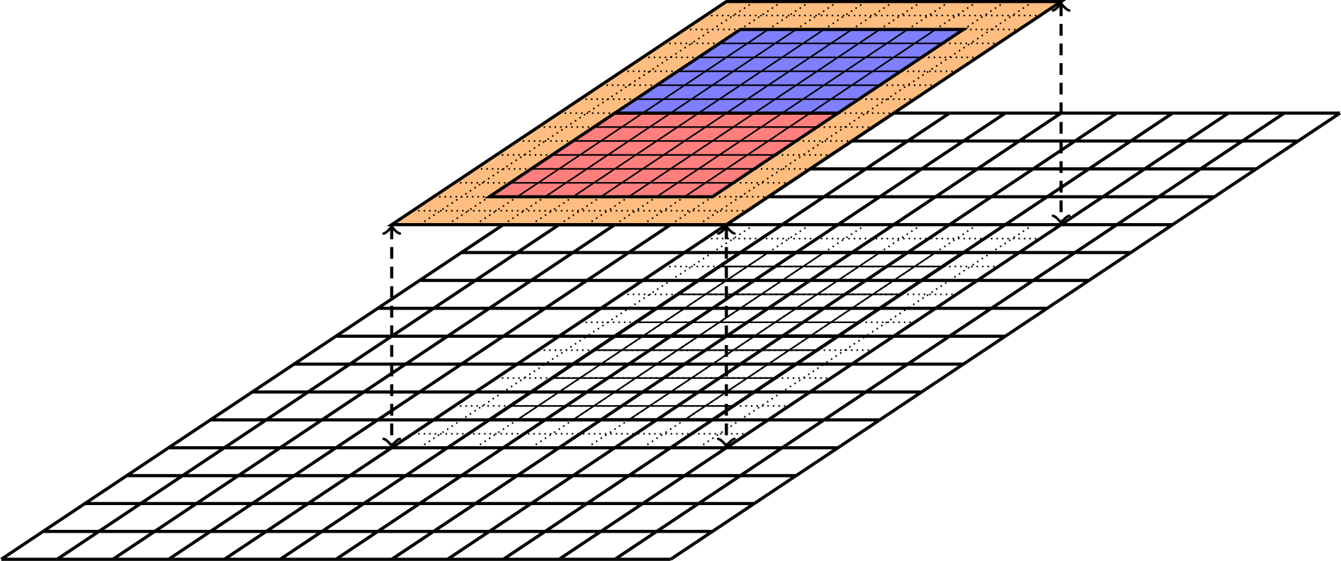
../_images/PatchBasedAMR.png — Fig. 9 Cartesian patch-based refinement showing two grid levels. The finer level consists of two patches (red and blue zones), and these zones each have a ghost cell layer 2 cells wide. The data lies on top of a coarse-grid data, i.e., data simultaneously exists on both the fine and the coarse levels. This data type is encapsulated by `EBAMRData<T>`.

The reason for having class encapsulation of mesh data is due to Realm, so that we can only keep track on which Realm the mesh data is defined. Users will interact with EBAMRData<T> through application code, or interacting with the core AMR functionality in AmrMesh (such as computing gradients, interpolating ghost cells etc.). AmrMesh has functionality for constructing most EBAMRData<T> types on a Realm, and EBAMRData<T> itself it typically not used anywhere elsewhere within chombo-discharge.

A number of explicit template specifications exist and are frequently used. These are outlined below:

typedef EBAMRData<EBCellFAB>        EBAMRCellData;  // Cell-centered single-phase data
typedef EBAMRData<EBFluxFAB>        EBAMRFluxData;  // Face-centered data in all coordinate direction
typedef EBAMRData<EBFaceFAB>        EBAMRFaceData;  // Face-centered in a single coordinate direction
typedef EBAMRData<BaseIVFAB<Real> > EBAMRIVData;    // Data on irregular data centroids
typedef EBAMRData<DomainFluxIFFAB>  EBAMRIFData;    // Data on domain phases
typedef EBAMRData<BaseFab<bool> >   EBAMRBool;      // For holding bool at every cell

typedef EBAMRData<MFCellFAB>        MFAMRCellData;  // Cell-centered multifluid data
typedef EBAMRData<MFFluxFAB>        MFAMRFluxData;  // Face-centered multifluid data
typedef EBAMRData<MFBaseIVFAB>      MFAMRIVData;    // Irregular face multifluid data

For example, EBAMRCellData is a Vector<RefCountedPtr<LevelData<EBCellFAB> > >, describing cell-centered data across the entire AMR hierarchy. There are many more data structures in place, but the above data structures are the most commonly used ones. Here, EBAMRFluxData is precisely like EBAMRCellData, except that the data is stored on cell faces rather than cell centers. Likewise, EBAMRIVData is a data holder that holds data on each EB centroid (or boundary centroid) across the entire AMR hierachy. In the same way, EBAMRIFData holds data on each face of all cut-cells in the hierarchy.

Allocating mesh data

To allocate data over a particular Realm, the user will interact with AmrMesh:

const int numComps = 1;
EBAMRCellData myData;
m_amr->allocate(myData, "myRealm", phase::gas, numComps);

Here, numCOmps determine the number of data components. Note that it does matter on which Realm and on which phase the data is defined. See Realm for details.

The user can specify a number of ghost cells for his/hers application code directly in the AmrMesh::allocate routine, like so:

int numComps = 1;
EBAMRCellData myData;
m_amr->allocate(myData, "myRealm", phase::gas, numComps, 5*IntVect::Unit);

If the user does not specify the number of ghost cells when calling AmrMesh::allocate, AmrMesh will use the default number of ghost cells specified in the input file.

Iterating over the AMR hierarchy

To iterate over data in an AMR hierarchy, you will first iterate over levels and then the patches on each level:

for (int lvl = 0; lvl < myData.size(); lvl++){
   LevelData<EBCellFAB>& levelData = *myData[lvl];

   const DisjointBoxLayout& levelGrids = levelData.disjointBoxLayout();

   for (DataIterator dit = levelGrids.dataIterator(); dit.ok(); ++dit){
      EBCellFAB& patchData = levelData[dit()];
   }
}

Throughout chombo-discharge it will be common to see the above implemented explicitly as a loop that supports OpenMP:

for (int lvl = 0; lvl < myData.size(); lvl++){
   LevelData<EBCellFAB>& levelData = *myData[lvl];

   const DisjointBoxLayout& levelGrids = levelData.disjointBoxLayout();
   const DataIterator& dataIterator    = levelGrids.dataIterator();

   const int numBoxes = dataIterator.size();

#pragma omp parallel for schedule(runtime)
   for (int currentBox = 0; currentBox < numBoxes; currentBox++) {
      const DataIndex& dataIndex = dataIterator[currentBox];

      EBCellFAB& patchData = levelData[dataIndex];
   }
}

Iterating over cells

For single-valued data, chombo-discharge uses standard loops (in column-major order) for iterating over data. For example, the standard loops for iterating over cell-centered data are

namespace BoxLoops {

   template <typename Functor>
   ALWAYS_INLINE void
   loop(const Box& a_computeBox, Functor&& kernel, const IntVect& a_stride = IntVect::Unit);

   template <typename Functor>
   ALWAYS_INLINE void
   loop(VoFIterator& a_iter, Functor&& a_kernel);
}

Here, the Functor argument is a C++ lambda or std::function which takes a grid cell as a single argument. For the first loop, we iterate over all grid cells in a_computeBox. Iterating over the cut-cells in a patch data holder (like the EBCellFAB) can be done with a VoFIterator, which can iterate through cells on an EBCellFAB that are not covered by the geometry. For example:

const int component = 0;

for (int lvl = 0; lvl < myData.size(); lvl++){
   LevelData<EBCellFAB>& levelData = *myData[lvl];

   const DisjointBoxLayout& levelGrids = levelData.disjointBoxLayout();

   for (DataIterator dit = levelGrids.dataIterator(); dit.ok(); ++dit){
      EBCellFAB& patchData       = levelData[dit()];
      BaseFab<Real>& regularData = patchData.getSingleValuedFab();

      auto regularKernel = [&](const IntVect& iv) -> void {
         regularData(iv, component) = 1.0;
      };

      auto irregularKernel = [&](const VolIndex& vof) -> void {
         patchData(vof, component = 1.0;
      };

      // Kernel regions (defined by user)
      Box computeBox = ...
      VoFIterator vofit = ...

      BoxLoops::loop(computeBox, regularKernel);
      BoxLoops::loop(vofit, irregularKernel);
   }
}

There are loops available for other types of data (e.g., face-centered data), see the BoxLoop documentation.

Coarsening data

Coarsening of data implies replacing the coarse-grid data that lies underneath a fine grid by some average of the fine-grid data. We currently support the following coarsening algorithms:

Arithmetic coarsening, in which the coarse-grid value is simply the average of the fine-grid values.
Conservative coarsening, in which the coarse-grid value is the conservative average of the fine-grid values. This implies that the total mass on the coarse-grid cell is identical to the total mass in the fine-grid cells from which one coarsened.
Harmonic, in which the coarse-grid value is the harmonic average of the fine-grid cell values.

These functions are available for both cell-centered data, cut-cell data, and face-centered data. Multiply signatures for this functionality exists, see the code-block below.

/*!
  @brief Average multifluid data over a specified realm
  @param[inout] a_data    Data to be coarsened.
  @param[in]    a_realm   Realm name
  @param[in]    a_average Averaging method
*/
void
average(MFAMRCellData& a_data, const std::string a_realm, const Average& a_average) const;

/*!
  @brief Average multifluid data over a specified realm
  @param[inout] a_data    Data to be coarsened.
  @param[in]    a_realm   Realm name
  @param[in]    a_average Averaging method
*/
void
average(MFAMRFluxData& a_data, const std::string a_realm, const Average& a_average) const;

/*!
  @brief Average down on specific realm and phase. 
  @param[inout] a_data  Data to be coarsened.
  @param[in]    a_realm Realm name
  @param[in]    a_phase Phase (gas or solid)
  @param[in]    a_average Averaging method
*/
void
average(EBAMRCellData&           a_data,
        const std::string        a_realm,
        const phase::which_phase a_phase,
        const Average&           a_average) const;

See the AmrMesh API for further details.

Filling ghost cells

Filling ghost cells is done using the interpGhost(...) functions in AmrMesh. This process adheres to the following rules:

Within a grid level, cells are always filled from neighboring grid patches without interpolation.
Around the halo zone (see Fig. 9), ghost cells are filled using slope-limited interpolation from the coarse grid only. Currently, this slope is calculated with a minmod limiter, although support for superbee, piecewise constant, and van Leer limiters are also implemented.

The signatures for updating the ghost cells are:

/*!
  @brief Interpolate ghost vectors over a realm, using the default ghost cell interpolation method. 
  @param[inout] a_data  Data to be interpolated.
  @param[in]    a_realm Realm name
  @param[in]    a_phase Phase (gas or solid)
*/
void
interpGhost(EBAMRCellData& a_data, const std::string a_realm, const phase::which_phase a_phase) const;

As one alternative, one can update ghost cells on a single grid level:

/*!
  @brief Interpolate ghost cells over a realm, using the default ghost cell interpolation method on a specific level. 
  @param[inout] a_fineData Fine grid data
  @param[inout] a_coarData Coarse grid data
  @param[in]    a_level    The grid level corresponding to a_fineData
  @param[in]    a_realm    Realm name
  @param[in]    a_phase    Phase (gas or solid)
*/
void
interpGhost(LevelData<EBCellFAB>&       a_fineData,
            const LevelData<EBCellFAB>& a_coarData,
            const int                   a_level,
            const std::string           a_realm,
            const phase::which_phase    a_phase) const;

Strictly speaking it is also possible to update ghost cells using the multigrid interpolator, but this will only fill a single layer of ghost cells around the halo zone (except near the cut-cells where additional cells are filled).

Interpolating from the coarse grid

Coarse-grid interpolation occurs, e.g., when the AMR hierarchy changes. If one needs data on a grid level where no data already exists, it is possible to fill this data by interpolating from the coarse grid to a finer one.

Important

This type of interpolation is distinctly different from the ghost cell interpolation, as it affects data across the whole grid patch.

The interpolation function that fill fine-grid data from a coarse grid has the following signature:

/*!
  @brief Interpolate data to new grids
  @details This is called when requiring data to be interpolated to new grids. Takes old data as argument
  and fills the new grid data with an interpolation of the old grid data. 
  @param[out] a_newData        New grid data.
  @param[in]  a_oldData        Old grid data.
  @param[in]  a_phase          Phase on which we regrid. 
  @param[in]  a_lmin           Coarsest level that did not change (but distribution may have changed). 
  @param[in]  a_oldFinestLevel Previous finest level.
  @param[in]  a_newFinestLevel New finest level. 
  @param[in]  a_type Interpolation type
*/
void
interpToNewGrids(EBAMRCellData&                   a_newData,
                 const EBAMRCellData&             a_oldData,
                 const phase::which_phase         a_phase,
                 const int                        a_lmin,
                 const int                        a_oldFinestLevel,
                 const int                        a_newFinestLevel,
                 const EBCoarseToFineInterp::Type a_type);

Here, the user must supply both the old data and the new data, as well as on which grid levels the interpolation will take place. The final argument a_type is the interpolation type. We currently support the following interpolation methods:

Type::PWC, which is piecewise-constant interpolation where the fine-cell data is filled with the coarse-cell values.
Type::ConservativePWC, which is a piecewise-constant interpolation that is also conservative (i.e., volume-weighted).
Type::ConservativeMinMod, which is a conservative interpolation method that uses the minmod limiter.
Type::ConservativeMonotonizedCentral, which is a conservative interpolation method that uses the van Leer limiter.
Type::Superbee, which is a conservative interpolation method that uses the superbeed limiter.

Note that there is “correct” interpolation method, but we note that we typically use a conservative minmod limiter in chombo-discharge.

Computing gradients

In chombo-discharge, gradients are computed using a standard second-order stencil based on finite differences. This is true everywhere except near the EB where the coarse-side stencil will avoid using the coarsened data beneath the fine level. This is shown in Fig. 10 which shows the typical 5-point stencil in regular grid regions, and also a much larger and more complex stencil.

In Fig. 10 we have shown two regular 5-point stencils (red and green). The coarse stencil (red) reaches underneath the fine level and uses the data defined by coarsening of the fine-level data. The coarsened data in this case is just a conservative average of the fine-level data. Likewise, the green stencil reaches over the refinement boundary and into one of the ghost cells on the coarse level.

Note

It is up to the user to ensure that ghost cells are filled prior to computing the gradient. This can be done either using multigrid interpolation (see Multigrid ghost cell interpolation), or standard interpolation (see Filling ghost cells).

Fig. 10 also shows a much larger stencil (blue stencil) on the coarse side of the refinement interface. The larger stencil is necessary because computing the \(y\) component of the gradient using a regular 5-point stencil would have the stencil reach underneath the fine level and into coarse data that is also irregular data. Since there is no unique way (that we know of) for coarsening the cut-cell fine-level data onto the coarse cut-cell without introducing spurious artifacts into the gradient, we reconstruct the gradient using a least squares procedure that entirely avoids using coarsened data. In this case we fetch a sufficiently large neighborhood of cells for computing a least squares minimization of a local solution reconstruction in the neighborhood of the coarse cell. In order to avoid fetching potentially badly coarsened data, this neighborhood of cells only uses valid grid cells, i.e., the stencil does not reach underneath the fine level at all. Once this neighborhood of cells is obtained, we compute the gradient using the procedure in Least squares.

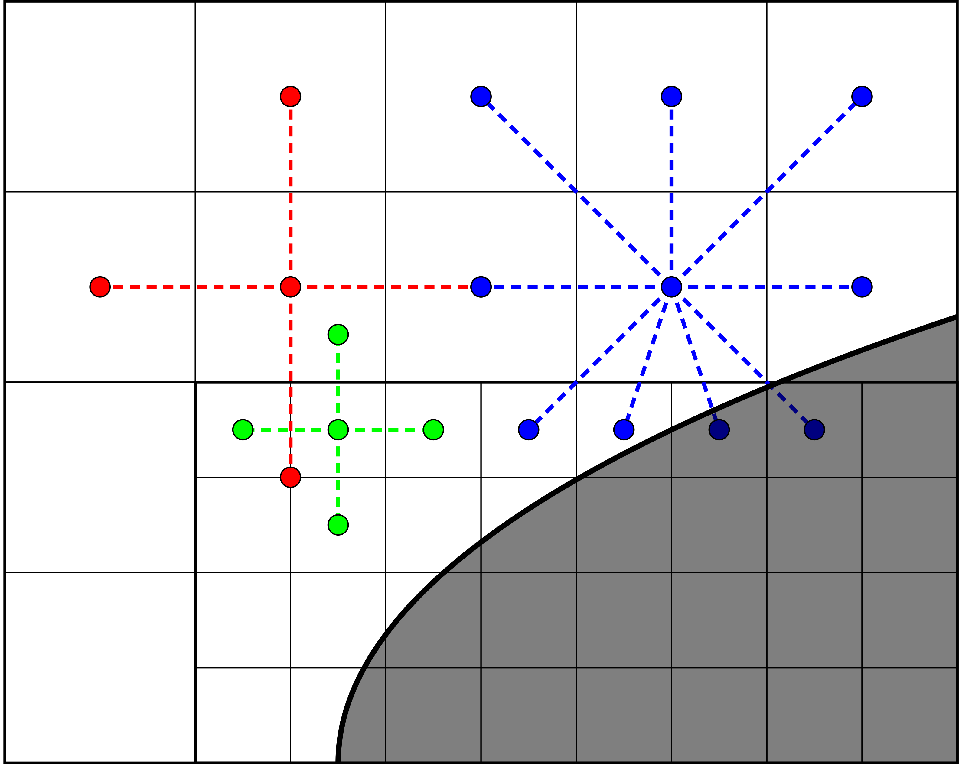
../_images/EBGradient.png — Fig. 10 Example of stencils for computing gradients near embedded boundaries. The red stencil shows a regular 5-point stencil for computing the gradient on the coarse side of the refinement boundary; it reaches into the coarsened data beneath the fine level. The green stencil shows a similar 5-point stencil on the fine side of the refinement boundary; the stencil reaches over the refinement boundary and into one ghost cell. The blue stencils shows a much more complex stencil which is computed using a least squares reconstruction procedure.

To compute gradients of a scalar, one can simply call AmrMesh::computeGradient(...) functions:

/*!
  @brief Compute cell-centered gradient over an AMR hierarchy. 
  @param[out] a_gradient Cell centered gradient. 
  @param[in]  a_phi      The scalar for which the gradient is computed. 
  @param[in]  a_realm    Name of the realm where the data lives. 
  @param[in]  a_phase    Phase on which the data lives. 
  @note This routine will reach into ghost cells and across refinement boundaries. The user must make sure that 
  ghost cells are updated before using this routine. 
*/
void
computeGradient(EBAMRCellData&           a_gradient,
                const EBAMRCellData&     a_phi,
                const std::string        a_realm,
                const phase::which_phase a_phase) const;

We reiterate that ghost cells must be updated before calling this routine. See AmrMesh or refer to the AmrMesh API for further details.

Copying data

To copy data between data holders, one may use the AmrMesh<T>::copyData(...) function or DataOps::copy (see DataOps).

The simplest way of copying data between data holders is via DataOps::copy, which does a local-only direct copy that also includes ghost cells. This version requires that the source and destination data holders are defined on the same realm, and does not invoke MPI calls.

A more general version is supplied by AmrMesh, and has the following structure:

/*!
  @brief Method for copying from a source container to a destination container. User supplies information
  @param[inout] a_dst        Destination data 
  @param[in]    a_src        Source data
  @param[in]    a_dstComps   Destination components
  @param[in]    a_srcComps   Source components
  @param[in]    a_toRegion   Region we copy into
  @param[in]    a_fromRegion Region we copy from
  @note If the user requests copying into ghosted regions, the Copiers MUST USE THE CORRECT NUMBER OF GHOST CELLS
  @note This routine will not work if copying between grids before/after regrids. 
*/
template <typename T>
void
copyData(EBAMRData<T>&       a_dst,
         const EBAMRData<T>& a_src,
         const Interval&     a_dstComps,
         const Interval&     a_srcComps,
         const CopyStrategy& a_toRegion   = CopyStrategy::Valid,
         const CopyStrategy& a_fromRegion = CopyStrategy::Valid) const noexcept;

In the above code, a_dst and a_src are the destination and source data holders for the copy. These need not be defined on the same Realm. Similarly, the a_dstComps and a_srcComps indicate the source and destination variables to be copied, which must have the same size. The final two arguments indicate which regions will be copied from. These are enums that are either CopyStrategy::Valid or CopyStrategy::ValidGhost, and indicates whether or not we will perform the copy only into valid cells (CopyStrategy::Valid) or also into the ghost cells (CopyStrategy::ValidGhost).

DataOps

We have prototyped functions for many common data operations in a static class DataOps.

Tip

For the full DataOps API, see the DataOps documentation.

DataOps contains numerous functions for operating on various template specializations of EBAMRData<T> (see Mesh data). For example, DataOps contains functions for scaling data, incrementing data, averaging cell-centered data onto faces, and many more.

Important

DataOps is designed to operate only within a single realm. This means that all arguments into the DataOps functions must be defined on the same realm.