Least squares

Least squares routines are useful for reconstructing a local polynomial in the vicinity of the embedded boundary. chombo-discharge supports the expansion of such solutions in a fairly general way. These routines are often needed because the embedded boundary introduces grid pathologies which are difficult to meet with pure finite differencing, see e.g. Ghost cell interpolation.

Polynomial expansion

Given some position $\mathbf{x}$, we expand the solution around a grid point $\mathbf{x}_{\mathbf{i}}$ to some order $Q$:

\[f\left(\mathbf{x}_{\mathbf{i}}\right) = f\left(\mathbf{x}_{\mathbf{i}}\right) + \nabla f\left(\mathbf{x}\right) \cdot \left(\mathbf{x}_{\mathbf{i}} - \mathbf{x}\right) + \ldots + \mathcal{O}\left(\Delta x^{Q+1}\right).\]

Using multi-index notation this is written as

\[f\left(\mathbf{x}_{\mathbf{i}}\right) = \sum_{|\alpha| \leq Q}\frac{\left(\mathbf{x}_{\mathbf{i}}-\mathbf{x}\right)^\alpha}{\alpha!} \left(\partial^\alpha f\right)\left(\mathbf{x}\right) + \mathcal{O}\left(\Delta x^{Q+1}\right),\]

where $\alpha$ is a multi-index. For a specified order $Q$ there is also a specified number of unknowns. E.g. in two dimensions with $Q = 1$ the unknowns are $f\left(\mathbf{x}\right)$, $\partial_x f\left(\mathbf{x}\right)$, and $\partial_y f\left(\mathbf{x}\right)$.

By expanding the solution around more grid points, we can formulate an over-determined system of equations $\mathbf{i} = 1, 2, 3, \ldots, N$ that allows us to compute the coefficients (i.e., unknowns) in the Taylor expansion. By using lexicographical ordering of the multi-indices, it is straightforward to write the system out explicitly. E.g., for $Q = 1$ in two dimensions:

\[\begin{split}\begin{pmatrix} 1 & (x_1 - x) & (y - y_1) \\ 1 & (x_2 - x) & (y - y_2) \\ \vdots & \ddots & \vdots \\ 1 & (x_N - x) & (y - y_N) \\ \end{pmatrix} \begin{pmatrix} f \\ \partial_x f \\ \partial_y f \\ \end{pmatrix}(\mathbf{x}) = \begin{pmatrix} f(\mathbf{x}_1) \\ f(\mathbf{x}_2) \\ \vdots \\ f(\mathbf{x}_N) \end{pmatrix}\end{split}\]

In general, we represent this system as

\[\mathbf{A}\mathbf{u} = \mathbf{b},\]

where unknowns in $\mathbf{u}$ are the coefficients in the Taylor series, ordered lexicographically (encoded with a Chombo IntVect). $\mathbf{b}$ is a column vector of grid point values representing the local expansion around each grid point, and $\mathbf{A}$ is the expansion matrix.

Note

chombo-discharge is not restricted to second order – it implements the above expansion to any order.

Neighborhood algorithm

To avoid reaching over or around embedded boundaries, the neighborhood algorithms only includes grid cells which can be reached by a monotone path. This path is defined by walking through neighboring grid cells without changing direction, see e.g. Fig. 34.

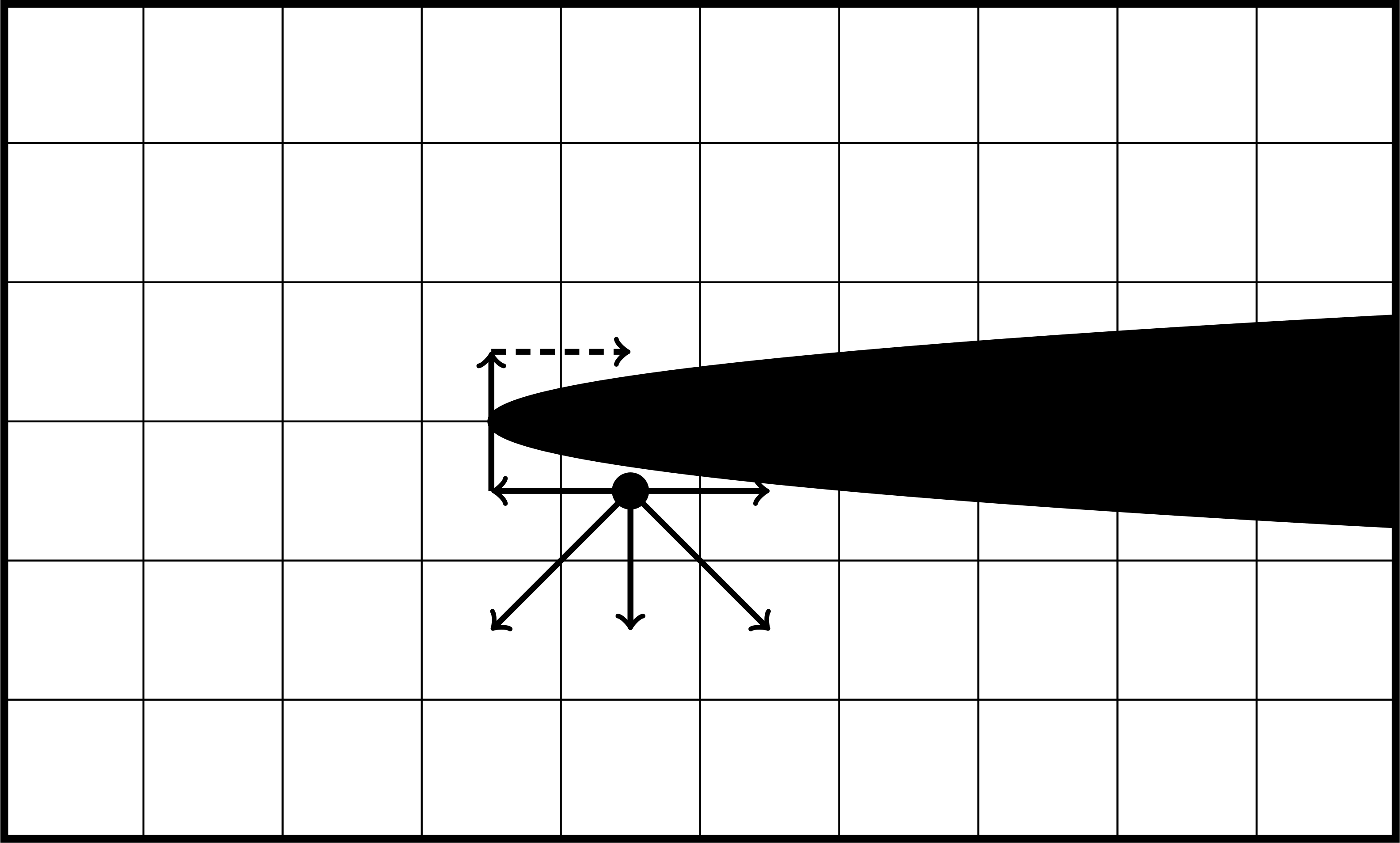
../_images/MonotonePath.png — Fig. 34 Neighborhood algorithm, only reaching into grid cells that can be reached by a monotone path. The grid cell at the end of the dashed line is excluded (even though it is a neighbor to the starting grid cell) since the path circulates the embedded boundary.

Weighted equations

Weights can also be added to each equation, e.g. to ensure that close grid points are more important than remote ones:

\[\begin{split}\begin{pmatrix} w_1 & w_1(x_1 - x) & w_N(y - y_1) \\ w_2 & w_2(x_2 - x) & w_N(y - y_2) \\ \vdots & \ddots & \vdots \\ w_N & w_N(x_N - x) & w_N(y - y_N) \\ \end{pmatrix} \begin{pmatrix} f \\ \partial_x f \\ \partial_y f \\ \end{pmatrix}(\mathbf{x}) = \begin{pmatrix} w_1f(\mathbf{x}_1) \\ w_2f(\mathbf{x}_2) \\ \vdots \\ w_Nf(\mathbf{x}_N) \end{pmatrix}\end{split}\]

For weighted least squares the system is represented as

\[\mathbf{W}\mathbf{A}\mathbf{u} = \mathbf{W}\mathbf{b},\]

where $\mathbf{W}$ are the weights. Typically, the weights are some power of the Euclidean distance

\[w_{\mathbf{i}} = \frac{1}{\left|\mathbf{x}_{\mathbf{i}} - \mathbf{x}\right|^p}.\]

Pseudo-inverse

An over-determined system does not have a unique solution, and so to obtain the solution to $\mathbf{u}$ for the system $\mathbf{W}\mathbf{A}\mathbf{u} = \mathbf{W}\mathbf{b}$ we use ordinary least squres. The solution is then

\[\mathbf{u} = \left[\left(\mathbf{W}\mathbf{A}\right)^+ \mathbf{W}\right]\mathbf{b},\]

where $\left(\mathbf{W}\mathbf{A}\right)^+$ is the Moore-Penrose inverse of $\mathbf{W}\mathbf{A}$. The pseudo-inverse is computed using the singular value decomposition (SVD) routines in LAPACK.

Note that the column vector $\mathbf{b}$ consist of known values (grid points), and the result $\left[\left(\mathbf{W}\mathbf{A}\right)^+ \mathbf{W}\right]$ can therefore be represented as a stencil. For example, in two dimensions with $Q = 1$ we find

\[\begin{split}\begin{pmatrix} f \\ \partial_x f \\ \partial_y f \end{pmatrix}(\mathbf{x}) = \begin{pmatrix} C_{11} & C_{12} & \ldots & C_{1N} \\ C_{21} & C_{22} & \ddots & C_{2N} \\ C_{31} & C_{32} & \ldots & C_{3N} \\ \end{pmatrix} \begin{pmatrix} f(\mathbf{x}_1) \\ f(\mathbf{x}_2) \\ \vdots \\ f(\mathbf{x}_N) \end{pmatrix}\end{split}\]

Pruning equations

If some terms in the Taylor series are specified, one can prune equations from the systems. E.g. if $f\left(\mathbf{x}\right)$ happens to be known, the system of equations can be rewritten as

\[\begin{split}\begin{pmatrix} w_1(x_1 - x) & w_N(y - y_1) \\ w_2(x_2 - x) & w_N(y - y_2) \\ \vdots & \vdots \\ w_N(x_N - x) & w_N(y - y_N) \\ \end{pmatrix} \begin{pmatrix} \partial_x f \\ \partial_y f \\ \end{pmatrix}(\mathbf{x}) = \begin{pmatrix} w_1f(\mathbf{x}_1) - w_1f(\mathbf{x}) \\ w_2f(\mathbf{x}_1) - w_2f(\mathbf{x}) \\ \vdots \\ w_Nf(\mathbf{x}_1) - w_Nf(\mathbf{x}) \\ \end{pmatrix}\end{split}\]

Again, following the benefits of lexicographical ordering it is straightforward to write an arbitrary order system of equations in the form $\mathbf{W}\mathbf{A}\mathbf{u} = \mathbf{W}\mathbf{b}$, even with an arbitrary number of terms pruned from the Taylor series. However, note that the result of the least squares solve is now in the format

\[\begin{split}\begin{pmatrix} \partial_x f \\ \partial_y f \end{pmatrix}(\mathbf{x}) = \begin{pmatrix} C_{11} & C_{12} & \ldots & C_{1N} \\ C_{21} & C_{22} & \ldots & C_{2N} \\ \end{pmatrix} \begin{pmatrix} f(\mathbf{x}_1) - f(\mathbf{x}) \\ f(\mathbf{x}_2) - f(\mathbf{x}) \\ \vdots \\ f(\mathbf{x}_N) - f(\mathbf{x}) \\ \end{pmatrix}.\end{split}\]

Thus, when evaluating the terms in the polynomial expansion the user must account for the modified right-hand side due to equation pruning. The modification to the right-hand side also depends on which terms are pruned from the expansion.

Source code

The source code for the least squares routines is found in $DISCHARGE_HOME/Source/Utilities/CD_LeastSquares.*, and the neighborhood algorithms are found in $DISCHARGE_HOME/Source/Utilities/CD_VofUtils.*.