Electrostatics model

The electrostatics model solves

\[\nabla\cdot\left(\epsilon_r\nabla\Phi\right) = -\frac{\rho}{\epsilon_0}\]

subject to the constraints and boundary conditions given in FieldSolver. The implementation is by a class

class FieldStepper : public TimeStepper

and is found in $DISCHARGE_HOME/Physics/Electrostatics. The C++ API is found here.

Solvers

This module uses the following solvers:

1. FieldSolver.

Time stepping

FieldStepper is a class with only stationary solves. This is enforced by making the TimeStepper::advance method throw an error, while the field solve itself is done in the initialization procedure in TimeStepper::postInitialize.

Important

To run the solver, one must set Driver.max_steps = 0.

Setting the space charge

Default behavior

By default, the initial space charge for this problem is given by Gaussian

\[\rho\left(\mathbf{x}\right) = \rho_0\exp\left(-\frac{\left|\mathbf{x}-\mathbf{x}_0\right|^2}{2R^2}\right),\]

where \(\rho_0\) is an amplitude, \(\mathbf{x}_0\) is the center and \(R\) is the Gaussian radius. These are set by the input options

FieldStepper.init_rho     = 1.0
FieldStepper.rho_center   = 0 0 0
FieldStepper.rho_radius   = 1.0

Custom value

For a more general way of specifying the space charge, FieldStepper has a public member function

void setRho(const std::function<Real(const RealVect& a_pos)>& a_rho, const phase::which_phase a_phase) noexcept;

Setting the surface charge

By default, the initial surface charge is set to a constant. This constant is given by

FieldStepper.init_sigma = 1.0

Custom value

For a more general way of specifying the surface charge, FieldStepper has a public member function

void setSigma(const std::function<Real(const RealVect& a_pos)>& a_sigma) noexcept;

Setting up a new problem

To set up a new problem, using the Python setup tools in $DISCHARGE_HOME/Physics/Electrostatics is the simplest way. To see available setup options, run

./setup.py --help

For example, to set up a new problem in $DISCHARGE_HOME/MyApplications/MyElectrostaticsProblem for a cylinder geometry, run

./setup.py -base_dir=MyApplications -app_name=MyElectrostaticsProblem -geometry=Cylinder

This will set up a new problem in a cylinder geometry (defined in Geometries/Cylinder).

Example programs

Some example programs for this module are given in

• $DISCHARGE_HOME/Exec/Examples/Electrostatics/Armadillo

• $DISCHARGE_HOME/Exec/Examples/Electrostatics/Mechshaft

• $DISCHARGE_HOME/Exec/Examples/Electrostatics/ProfiledSurface

Verification

Spatial convergence tests for this module (and consequently the underlying numerical discretization) are given in

• $DISCHARGE_HOME/Exec/Convergence/Electrostatics/C1

• $DISCHARGE_HOME/Exec/Convergence/Electrostatics/C2

• $DISCHARGE_HOME/Exec/Convergence/Electrostatics/C3

All tests operate by computing solutions on grids with resolutions \(\Delta x\) and \(\Delta x/2\) and then computing the solution error using the approach outlined in Spatial convergence.

C1: Coaxial cable

$DISCHARGE_HOME/Exec/Convergence/Electrostatics/C1 is a spatial convergence test in a coaxial cable geometry. Figure Fig. 28 shows the field distribution. Note that there is a dielectric embedded between the two cylindrical shells.

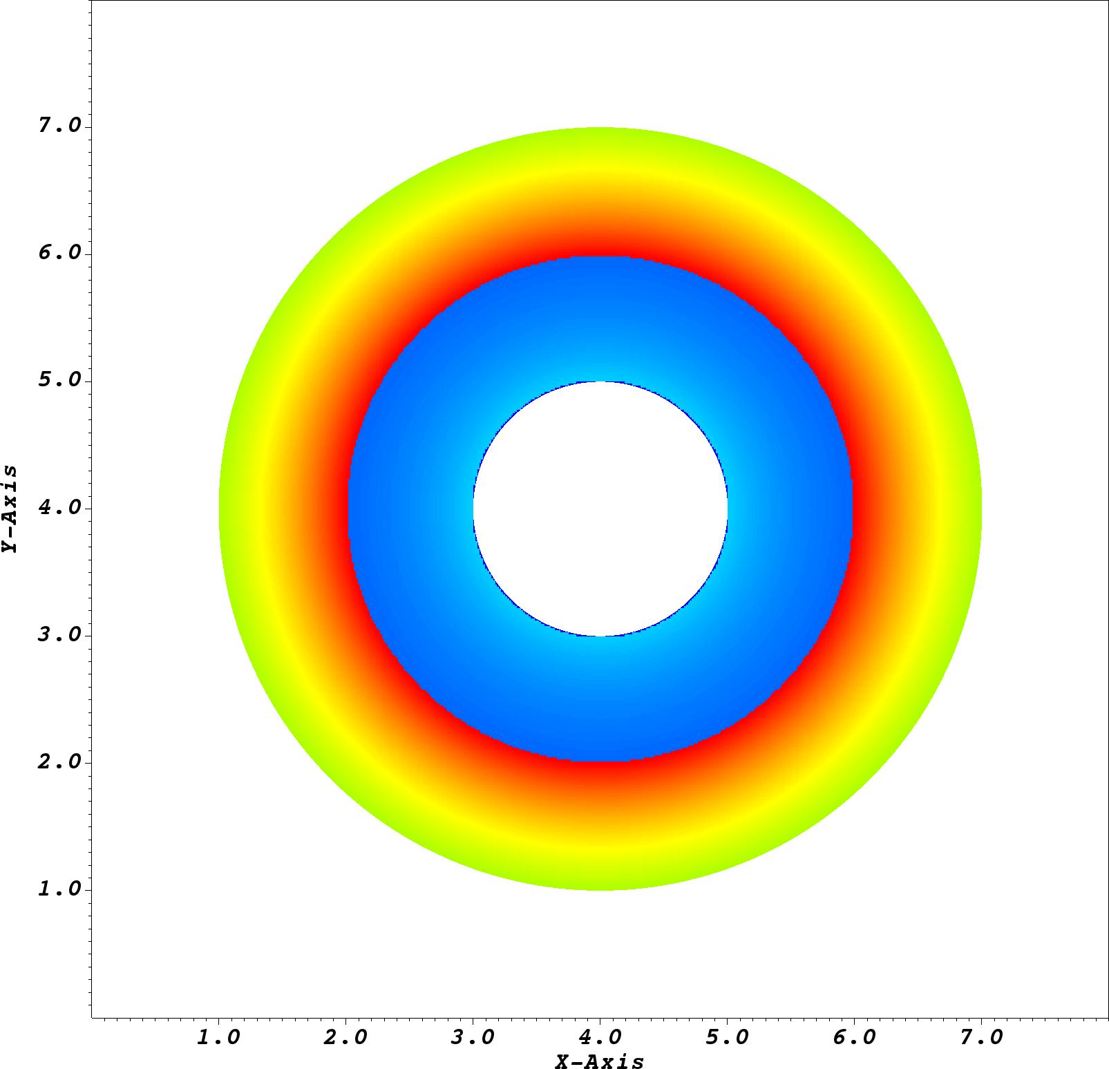
Fig. 28 Field distribution for a coaxial cable geometry on a \(512^2\) grid.

The computed convergence rates are given in Fig. 29. We find second order convergence in all three norms.

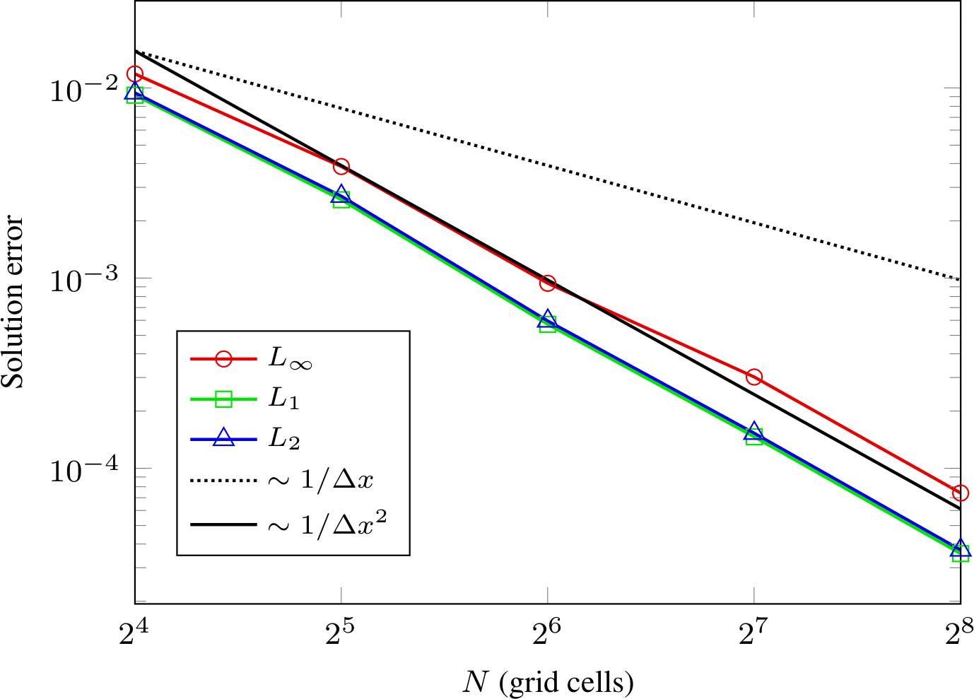
Fig. 29 Spatial convergence rates for two-dimensional coaxial cable geometry.

C2: Profiled surface

$DISCHARGE_HOME/Exec/Convergence/Electrostatics/C2 is a 2D spatial convergence test for an electrode and a dielectric slab with surface profiles. Figure Fig. 30 shows the field distribution.

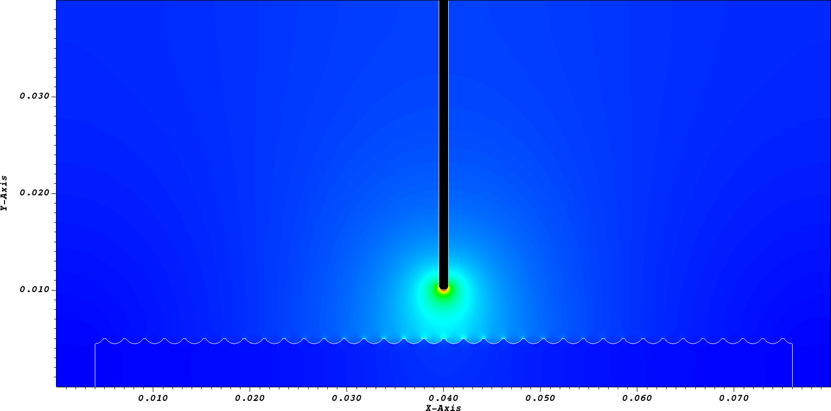
Fig. 30 Field distribution for a profiled surface geometry on a \(2048^2\) grid.

The computed convergence rates are given in Fig. 31. We find second order convergence in all three norms.

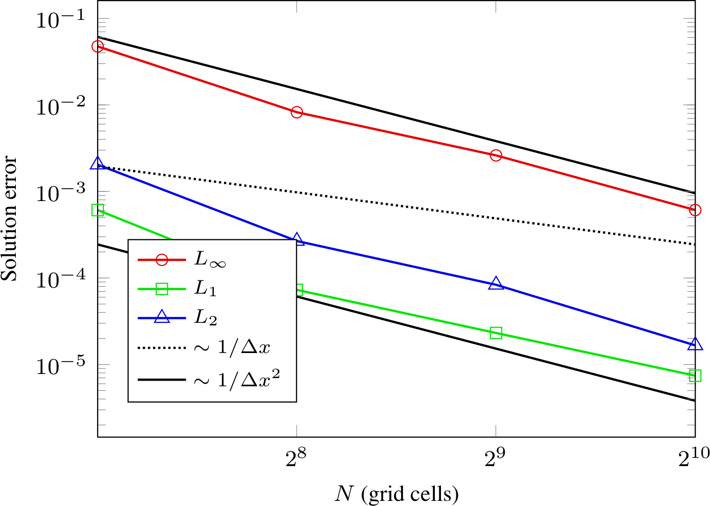
Fig. 31 Spatial convergence rates for two-dimensional dielectric surface profile.

C3: Dielectric shaft

$DISCHARGE_HOME/Exec/Convergence/Electrostatics/C3 is a 3D spatial convergence test for a dielectric shaft perpendicular to the background field. Figure Fig. 32 shows the field distribution for a \(256^3\) grid.

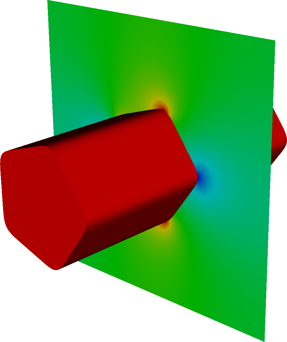
Fig. 32 Field distribution for a profiled surface geometry on a \(256^3\) grid.

The computed convergence rates are given in Fig. 33. We find second order convergence in \(L_1\) and \(L_2\) on all grids, and find second order convergence in the max-norm on sufficiently fine grids. On coarser grids, the reduced convergence rate in the max-norm is probably due to under-resolution of the geometry.

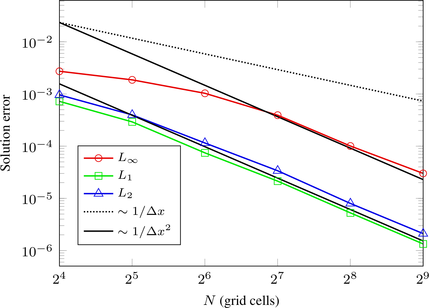
Fig. 33 Spatial convergence rates.