Linear solvers

Helmholtz equation

The Helmholtz equation is represented by

\[\alpha a\left(\mathbf{x}\right)\Phi + \beta\nabla\cdot\left[b\left(\mathbf{x}\right)\nabla\Phi\right] = \rho\]

where $\alpha$ and $\beta$ are constants and $a\left(\mathbf{x}\right)$ and $b\left(\mathbf{x}\right)$ are spatially dependent and piecewise smooth.

To solve the Helmholtz equation, it is solved in the form

\[\kappa L\Phi = \kappa\rho,\]

where $L$ is the Helmholtz operator above. The preconditioning by the volume fraction $\kappa$ is done in order to avoid the small-cell problem encountered in finite-volume discretizations on EB grids.

Discretization and fluxes

The Helmholtz equation is solved by assuming that $\Phi$ lies on the cell-center. The $b\left(\mathbf{x}\right)$-coefficient is defined on face centers and EB faces, while $a\left(\mathbf{x}\right)$ is defined on cell centers. In the general case the cell center might lie inside the embedded boundary, and the cell-centered discretization relies on the concept of an extended state. Thus, $\Phi$ does not satisfy a discrete maximum principle.

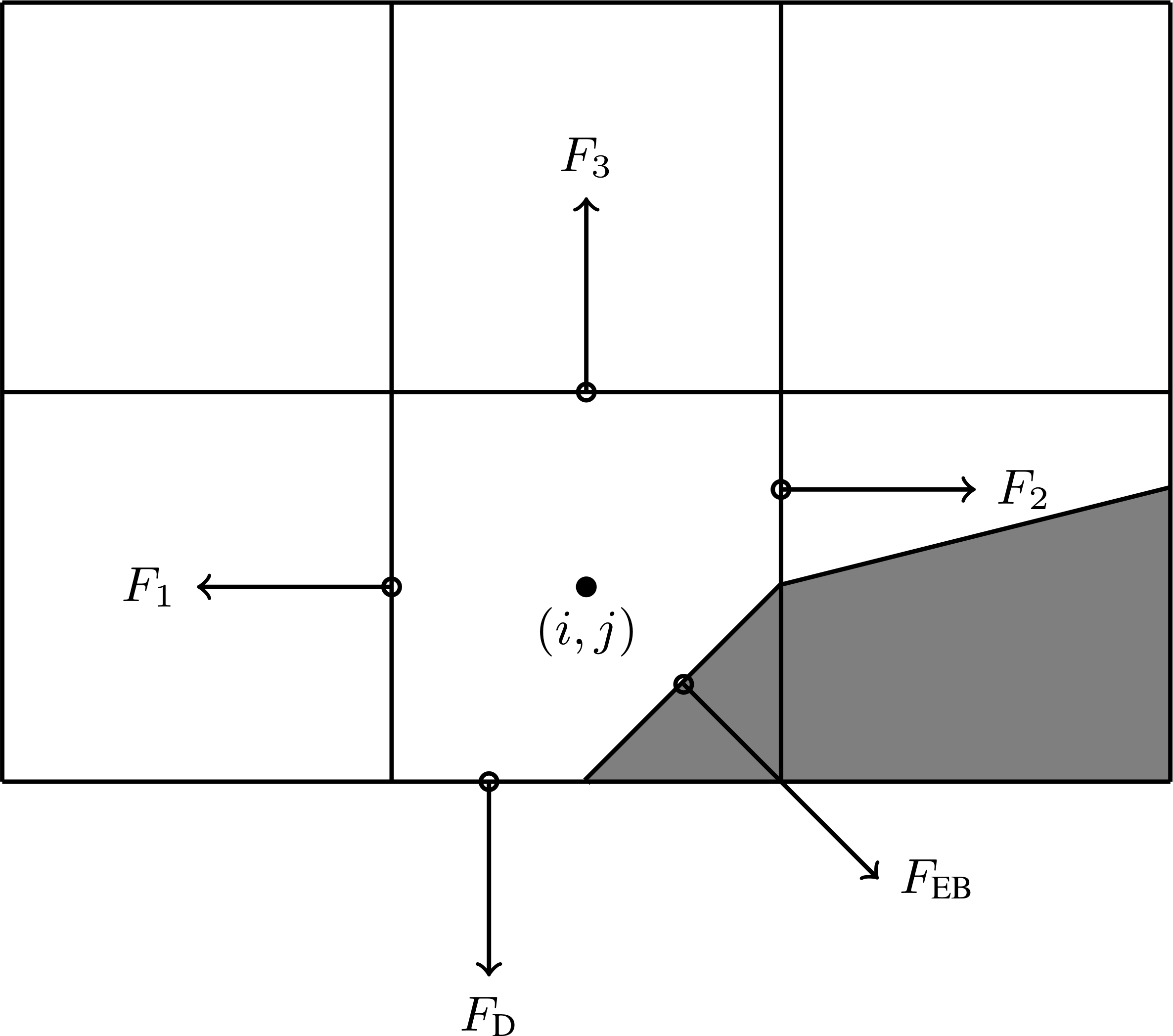
../_images/CutCell.png — Fig. 16 Location of fluxes for finite volume discretization.

The finite volume update require fluxes on the face centroids rather than the centers. These are constructed by first computing the fluxes to second order on the face centers, and then interpolating them to the face centroids. For example, the flux $F_3$ in the figure above is

\[F_3 = \beta b_{i,j+1/2}\frac{\Phi_{i,j+1} - \Phi_{i,j}}{\Delta x}.\]

The other fluxes, such as $F_2$ requires interpolation of face-centered fluxes to the face centroids.

Boundary conditions

The finite volume discretization of the Helmholtz equation require fluxes through the EB and domain faces. Below, we discuss how these are implemented.

Note

chombo-discharge supports spatially dependent boundary conditions

Neumann

Neumann boundary conditions are straightforward since the flux through the EB or domain faces are specified directly. I.e., the fluxes $F_{\textrm{EB}}$ and $F_{\textrm{D}}$ are directly specified in Fig. 16.

Dirichlet

Dirichlet boundary conditions are more involved since only the value at the boundary is prescribed, but the finite volume discretization requires a flux. On the domain boundaries where there is no EB the fluxes are face-centered and we therefore use finite differencing for obtaining a second order accurate approximation to the flux at the boundary. If the EB intersects the domain side, we interpolate face-centered fluxes to face centroids.

On the embedded boundaries the flux is more complicated to compute, and requires us to compute an approximation to the normal gradient $\partial_n\Phi$ at the boundary. Our approach is to approximate this flux by expanding the solution as a polynomial using a specified number of grid cells. By using more grid cells than there are unknown in the Taylor series, we formulate an over-determined system of equations up to some specified order. As a first approximation we include only those cells in the quadrant or half-space defined by the normal vector, see Fig. 17. If we can not find enough equations, several fallback options are in place to ensure that we obtain a sufficient number of equations.

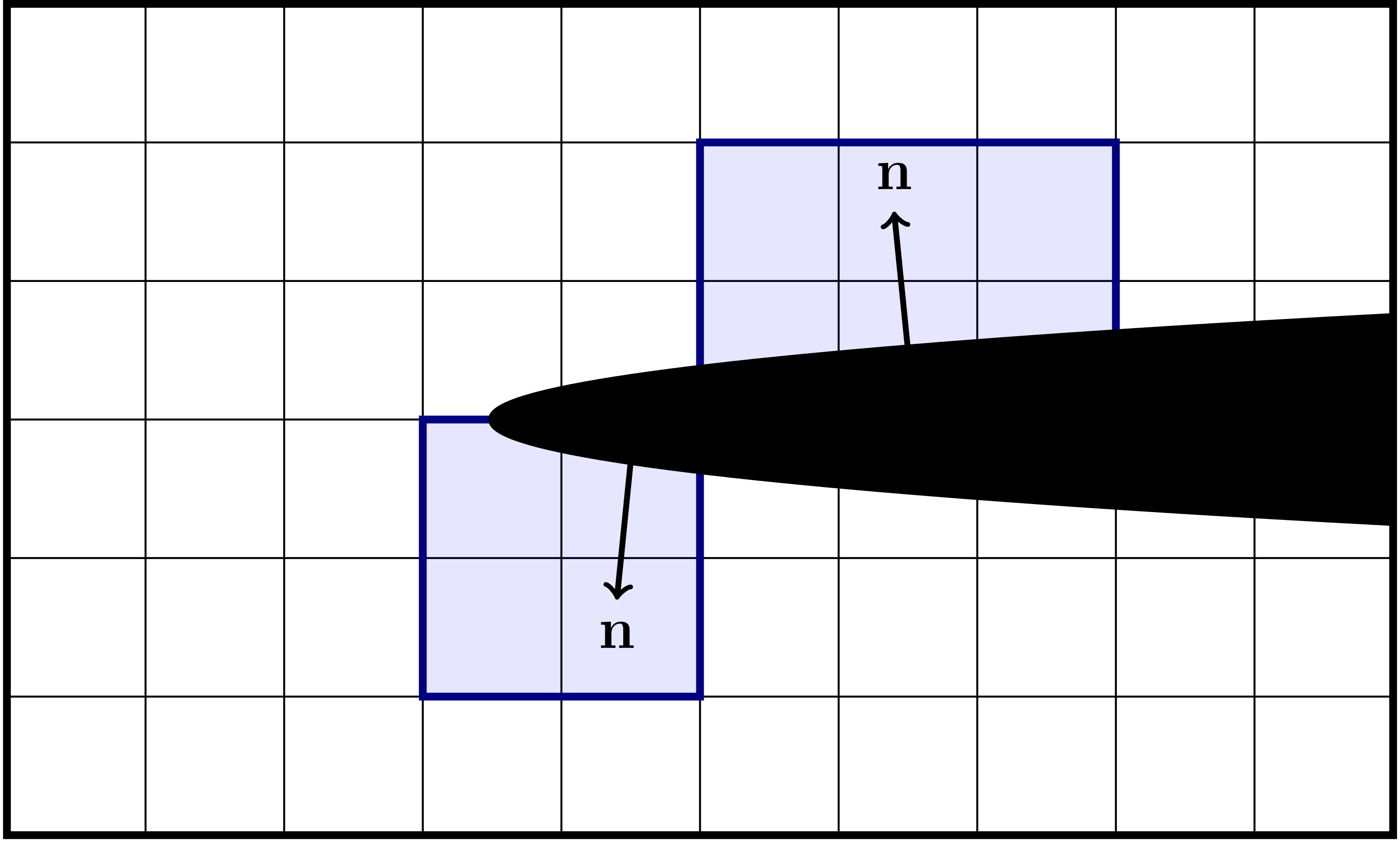
../_images/GradientReconstruction.png — Fig. 17 Examples of neighborhoods (quadrant and half-space) used for gradient reconstruction on the EB.

Once the cells used for the gradient reconstruction have been obtained, we use weighted least squares to compute the approximation to the derivative to specified order (for details, see Least squares). The result of the least squares computation is represented as a stencil:

\[\frac{\partial\Phi}{\partial n} = w_{\textrm{B}}\Phi_{\textrm{B}} + \sum_{\mathbf{i}} w_{\mathbf{i}}\Phi_{\mathbf{i}},\]

where $\Phi_{\textrm{B}}$ is the value on the boundary, the $w$ are weights for grid points $\mathbf{i}$, and the sum runs over cells in the domain.

Note that the gradient reconstruction can end up requiring more than one ghost cell layer near the embedded boundaries. For example, Fig. 18 shows a typical stencil region which is built when using second order gradient reconstruction on the EB. In this case the gradient reconstruction requires a stencil with a radius of 2, but as the cut-cell lies on the refinement boundary the stencil reaches into two layers of ghost cells. For the same reason, gradient reconstruction near the cut-cells might require interpolation of corner ghost cells on refinement boundaries.

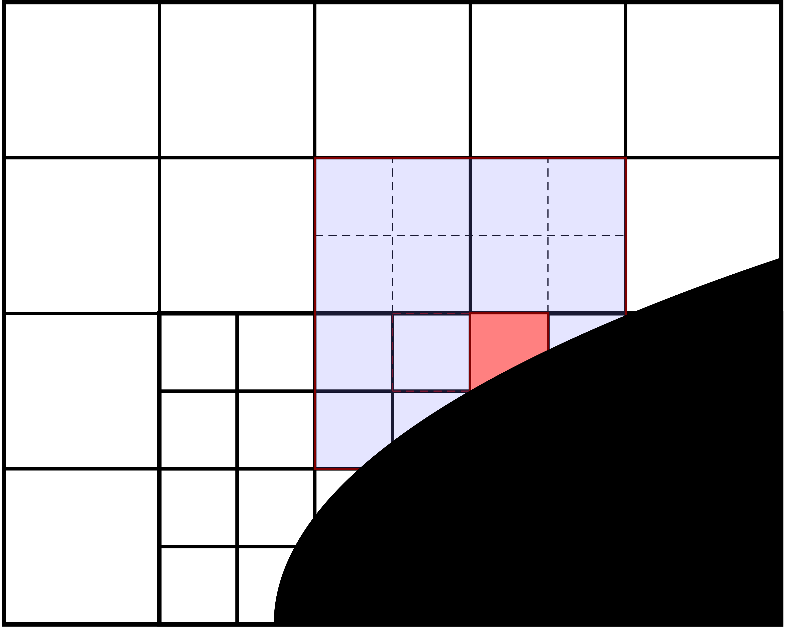
../_images/StencilRegion.png — Fig. 18 Example of the region of a second order stencil for the Laplacian operator with second order gradient reconstruction on the embedded boundary.

Here, we rely on multigrid interpolation (see Multigrid ghost cell interpolation) to fill the required number of ghost cells.

Robin

Robin boundary conditions are in the form

\[A\partial_n\Phi + B\Phi = C,\]

where $A$, $B$, and $C$ are constants. This boundary conditions is enforced through the flux

\[\partial_n\Phi = \frac{1}{A}\left(C - B\Phi\right),\]

which requires an evaluation of $\Phi$ on the domain boundaries and the EB.

For domain boundaries we extrapolate the cell-centered solution to the domain edge, using standard first order finite differencing.

On the embedded boundary, we approximate $\Phi\left(\mathbf{x}_{\text{EB}}\right)$ by linearly interpolating the solution with a least squares fit, using cells which can be reached with a monotone path of radius one around the EB face (see Least squares for details). The Robin boundary condition takes the form

\[\partial_n\Phi = \frac{C}{A} - \frac{B}{A}\sum_{\mathbf{i}} w_{\mathbf{i}}\Phi_{\mathbf{i}}.\]

Currently, we include the data in the cut-cell itself in the interpolation (and thus also use unweighted least squares to avoid forming an ill-conditioned system).

Multigrid ghost cell interpolation

With AMR, multigrid requires ghost cells on the refinement boundary. The interior stencils for the Helmholtz operator have a radius of one and thus only require a single layer of ghost cells (and no corner ghost cells). These ghost cells are filled using a finite-difference stencil, see Fig. 19.

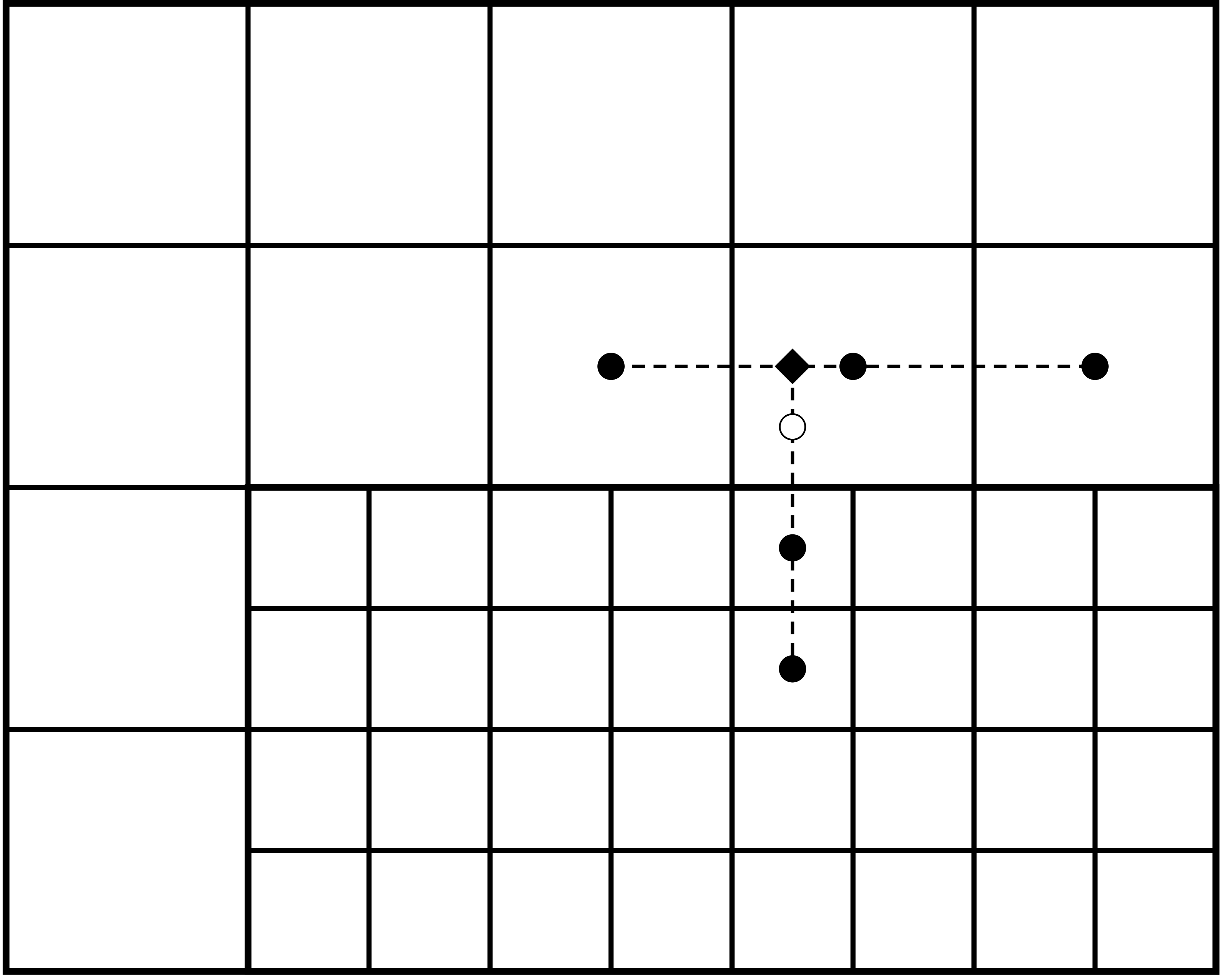
../_images/MultigridInterpolation.png — Fig. 19 Standard finite-difference stencil for ghost cell interpolation (open circle). We first interpolate the coarse-grid cells to the centerline (diamond). The coarse-grid interpolation is then used together with the fine-grid cells (filled circles) for interpolation to the ghost cell (open circle).

Embedded boundaries introduce many pathologies for multigrid:

Cut-cell stencils may have a large radius (see Fig. 18) and thus require more ghost cell layers.
The EBs cut the grid in arbitrary ways, leading to multiple pathologies regarding cell availability.

The pathologies mean that standard finite differencing fails near the EB, mandating a more general approach. Our way of handling ghost cell interpolation near EBs is to reconstruct the solution (to specified order) in the ghost cells, using the available cells around the ghost cell (see Least squares for details). As per conventional wisdom regarding multigrid interpolation, this reconstruction does not use coarse-level grid cells that are covered by the fine level.

Figure Fig. 20 shows a typical interpolation stencil for the stencil in Fig. 18. Here, the open circle indicates the ghost cell to be interpolated, and we interpolate the solution in this cell using neighboring grid cells (closed circles). For this particular case there are 10 nearby grid cells available, which is sufficient for second order interpolation (which requires at least 6 cells in 2D).

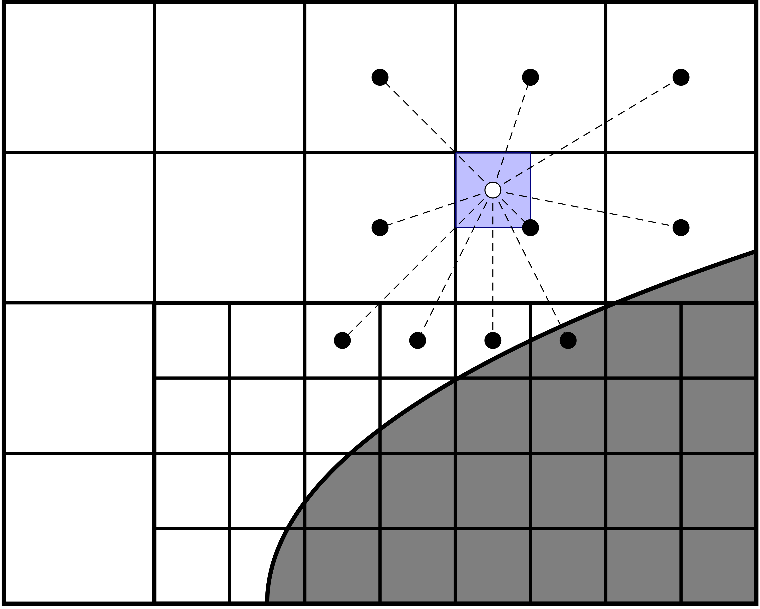
../_images/EBMultigridInterpolation.png — Fig. 20 Multigrid interpolation for refinement boundaries away from and close to an embedded boundary.

Note

chombo-discharge implements a fairly general ghost cell interpolation scheme near the EB. The ghost cell values can be reconstructed to specified order (and with specified least squares weights).

Relaxation methods

The Helmholtz equation is solved using multigrid, with various smoothers available on each grid level. The currently supported smoothers are:

Standard point Jacobi relaxation.
Red-black Gauss-Seidel relaxation in which the relaxation pattern follows that of a checkerboard.
Multi-colored Gauss-Seidel relaxation in which the relaxation pattern follows quadrants in 2D and octants in 3D.

Users can select between the various smoothers in solvers that use multigrid.

Tip

Red-black Gauss-Seidel usually provide the best convergence rates. The multi-colored kernels are twice as expensive as red-black Gauss-Seidel relaxation in 2D, and four times as expensive in 3D, and then to only marginally improve convergence rates.

Multiphase Helmholtz equation

chombo-discharge also supports a multiphase version where data exists on both sides of the embedded boundary. The most common case is that involving discontinuous coefficients across the EB, e.g. for

\[\beta\nabla\cdot\left[b\left(\mathbf{x}\right)\nabla\Phi\left(\mathbf{x}\right)\right] = \rho.\]

where $b\left(\mathbf{x}\right)$ is only piecewise constant. This is the natural boundary conditions on a dielectric surface, for example.

Jump conditions

For the case of discontinous coefficients there is a jump condition on the interface between two materials:

(4)\[b_1\partial_{n_1}\Phi + b_2\partial_{n_2}\Phi = \sigma,\]

where $b_1$ and $b_2$ are the Helmholtz equation coefficients on each side of the interface, and $n_1 = -n_2$ are the normal vectors pointing away from the interface in each phase. The jump factor is $\sigma$, and can be thought of as the surface charge density on the dielectric.

Discretization

To incorporate the jump condition in the Helmholtz discretization, we use a gradient reconstruction to obtain an approximation of $\Phi$ on the boundary, using Eq. 4. We then use this value to impose a Dirichlet boundary condition during multigrid relaxation. Recalling the gradient reconstruction $\frac{\partial\Phi}{\partial n} = w_{\textrm{B}}\Phi_{\textrm{B}} + \sum_{\mathbf{i}} w_{\mathbf{i}}\Phi_{\mathbf{i}}$, the matching condition (see Fig. 21) can be written as

\[b_1\left[w_{\textrm{B},1}\Phi_{\textrm{B}} + \sum_{\mathbf{i}} w_{\mathbf{i},1}\Phi_{\mathbf{i},1}\right] + b_2\left[w_{\textrm{B},2}\Phi_{\textrm{B}} + \sum_{\mathbf{i}} w_{\mathbf{i},2}\Phi_{\mathbf{i},2}\right] = \sigma.\]

This equation can be solved for the boundary value $\Phi_{\textrm{B}}$, which can then be used to compute the finite-volume fluxes into the cut-cells.

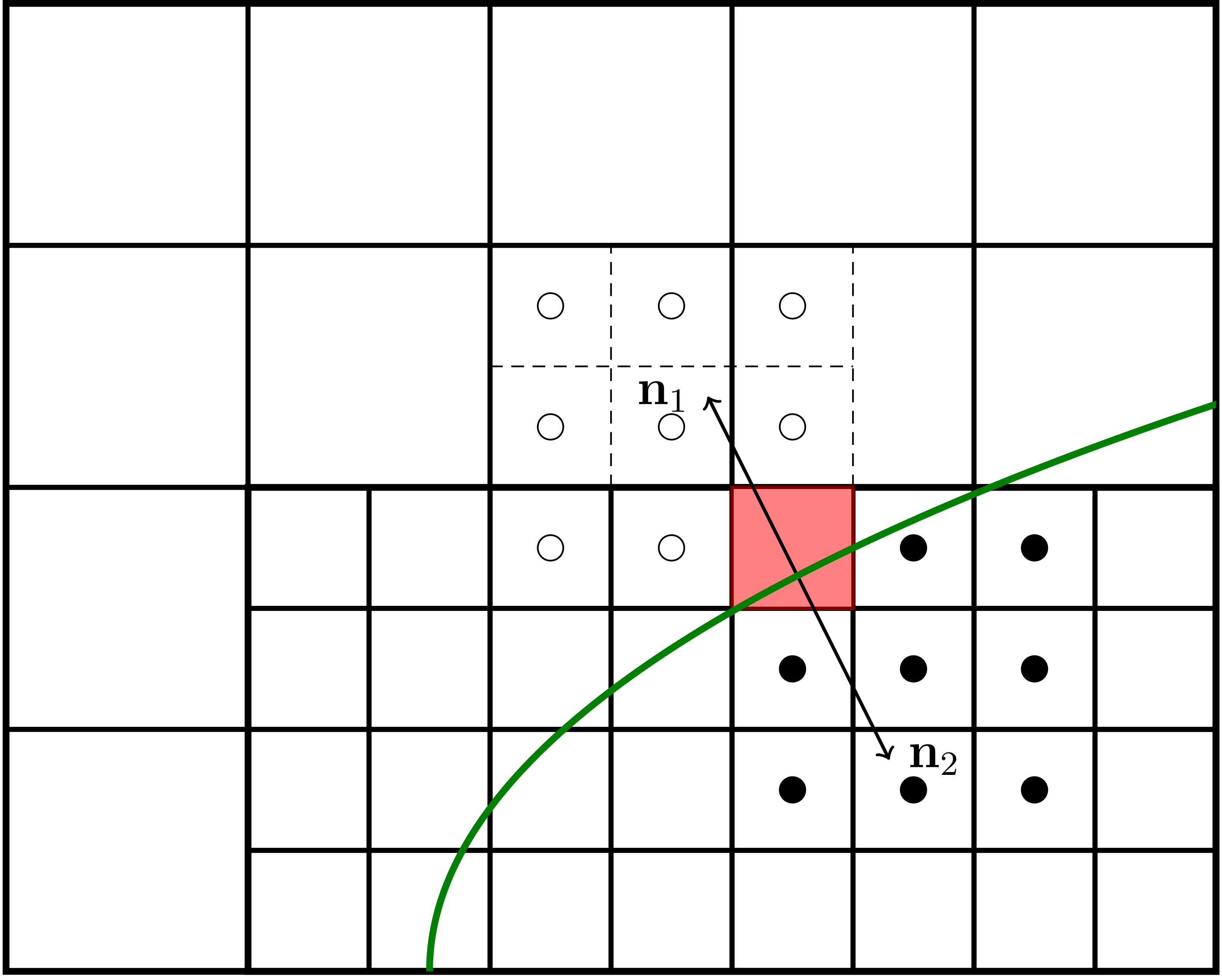
../_images/JumpCondition.png — Fig. 21 Example of cells and stencils that are involved in discretizing the jump condition. Open and filled circles indicate cells in separate phases.

Note

For discontinuous coefficients the gradient reconstruction on one side of the EB does not reach into the other (since the solution is not differentiable across the EB).

AMRMultiGrid

AMRMultiGrid is the Chombo implementation of the Martin-Cartwright multigrid algorithm. It takes an “operator factory” as an argument, and the factory can generate objects (i.e., operators) that encapsulate the discretization on each AMR level.

chombo-discharge uses its own elliptic operators, and the user can use either of:

EBHelmholtzOpFactory for single-phase problems.
MFHelmholtzOpFactory for multi-phase problems.

The source code for these are located in $DISCHARGE_HOME/Source/Elliptic.

Bottom solvers

Chombo provides (at least) three bottom solvers which can be used with AMRMultiGrid.

A regular smoother (e.g., point Jacobi).
A biconjugate gradient stabilized method (BiCGStab)
A generalized minimal residual method (GMRES).

The user can select between these for the various solvers that use multigrid. Typically, smoothers tend to work sufficiently well but improved convergence rates can occasionally be achieved by using a conjugate gradient solver.