Kinetic Monte Carlo

Concept

Kinetic Monte Carlo solvers advance a state (or multiple states) represented e.g. as state vectors

\[\begin{split}\vec{X}(t) = \begin{pmatrix} X_1(t) \\ X_2(t) \\ X_3(t) \\ \vdots \end{pmatrix}\end{split}\]

Each row in $\vec{X}$ represents e.g. the population of some chemical species. Reactions between species are represented stoichiometrically as

\[X_A + X_B + \ldots \xrightarrow{k} X_C + X_D + \ldots,\]

where $k$ is the reaction rate. Each such reaction is associated with a state change in $\vec{X}$, e.g.

\[\vec{X}\xrightarrow{r} \vec{X} + \vec{\nu}_r,\]

where $r$ is the reaction type and $\nu_r$ is the state change associated with the firing of one reaction of type $r$. A set of such reactions is called the reaction network $\vec{R}$.

Propensities $a_r\left(\vec{X}\right)$ are defined such that $a_r\left(\vec{X}\right)\textrm{d}t$ is the probability that exactly one reaction of type $r$ occurs in the time interval $[t, t+\textrm{d}t]$. For unimolecular reactions of the type

\[X_A + X_B + \ldots \xrightarrow{k} \emptyset\]

with $A \neq B \neq \ldots$ the propensity function is $k X_A X_B \ldots$. For bimolecular of the type

\[2X_A \xrightarrow{k} \emptyset\]

the propensity is $k \frac{1}{2} X_A(X_A-1)$ because there are $\frac{1}{2}X_A(X_A-1)$ unique pairs of molecules of type A. Propensities for higher-order reactions can then be expanded using the binomial theorem. For example, for a third-order reaction $3X_A\xrightarrow{k} \emptyset$ the propensity function is $k\frac{1}{6}X_A(X_A-1)(X_A-2)$.

Various algorithms can be used for advancing the state $\vec{X}$ for an arbitrary reaction network $\vec{R}$.

The Stochastic simulation algorithm (SSA). The SSA is also known as the Gillespie algorithm [Gillespie, 1977], and is an exact stochastic solution to the above problem. However, it becomes inefficient as the number of reactions per unit time grows.
Tau leaping, which is an approximation to the SSA which uses Poisson sampling of the underlying reactions.
Hybrid advance, see Hybrid algorithm. The hybrid algorithm is taken from Cao et al. [2006], and switches between tau leaping and the SSA in their respective limits.

Stochastic simulation algorithm

For the SSA we compute the time until the next reaction by

\[T = \frac{1}{\sum_{r\in\vec{R}} a_r}\ln\left(\frac{1}{u_1}\right)\]

where $A = \sum_{r\in\vec{R}} a_r$ and $u_1$ is a uniformly distributed random variable between $0$ and $1$. The type of reaction that fires is deterimined from

\[r_c = \textrm{smallest integer satisfying } \sum_{r^\prime = 1}^{r_c} a_{r^\prime} > u_2A,\]

where and $u_2$ is another uniformly distributed random variable between $0$ and $1$. The state is then advanced as

\[\vec{X}(t+T) = \vec{X}(t) + \vec{\nu}_{r_c}.\]

Tau leaping

With tau-leaping the state is advanced over a time $\Delta t$ as

\[\vec{X}\left(t+\Delta t\right) = \vec{X}\left(t\right) + \sum_{\vec{R}} \vec{\nu}_r\mathcal{P}\left(a_r\left[\vec{X}\left(t\right)\right]\Delta t\right),\]

where $\mathcal{P}$ is a Poisson-distributed random variable. Note that tau leaping may fail to give a thermodynamically valid state, and should thus be used in combination with step rejection.

Hybrid algorithm

The hybrid algorithm is taken from Cao et al. [2006]. Assume that we wish to integrate over some time $\Delta t$, which proceeds as follows:

Let $\tau = 0$ be the simulated time within $\Delta t$.
Partition the reaction set $\vec{R}$ into critical and non-critical reactions. The critical reactions are defined as the subset of $\vec{R}$ that are within $N_{\textrm{crit}}$ firings away from exhausting one of its reactants. The non-critical reactions are defined as the remaining subset.
Compute time steps until the firing of the next critical reaction, and a time step such that the propensities of the non-critical reactions do not change by more than some relative factor $\epsilon$. Let these time steps be given by $\Delta \tau_{\textrm{c}}$and $\Delta \tau_{\textrm{nc}}$.
Select a reactive substep within $\Delta t$ from

\[\Delta \tau = \min\left[\Delta t - \tau, \min\left(\Delta \tau_{\textrm{c}}, \Delta \tau_{\textrm{nc}}\right)\right]\]
Resolve reactions as follows:
1. If $\Delta \tau_{\textrm{c}} < \Delta \tau_{\textrm{nc}}$ and $\Delta \tau_{\textrm{c}} < \Delta t - \tau$ then one critical reaction fires. Determine the reaction type using the SSA algorithm.
  
  Next, advance the state using tau leaping for the non-critical reaction.
2. Otherwise: No crical reactions fire. Advance the state using tau-leapnig for the non-critical reactions only. An exception is made if $A\Delta\tau$ is smaller than some specified threshold in which case we switch to SSA advancement (which is more efficient in this limit).
Check if $\vec{X}$ is a thermodynamically valid state.
1. If the state is valid, accept it and let $\tau \rightarrow \tau + \Delta\tau$.
2. If the state is invalid, reject the advancement. Let $\Delta\tau_{\textrm{nc}} \rightarrow \Delta \tau_{\textrm{nc}}/2$ and return to step 4).
If $\tau < \Delta t$, return to step 2.

The Cao et al. [2006] algorithm requires algorithmic specifications as follows:

The factor $\epsilon$ which determines the non-critical time step.
The factor $N_{\textrm{crit}}$ which determines which reactions are critical or not.
Factors for determining when and how to switch to the SSA-based algorithm in step 5b.

Implementation

The Kinetic Monte Carlo solver is implemented as

template <typename R, typename State, typename T = long long>
class KMCSolver
{
public:
   using ReactionList = std::vector<std::shared_ptr<const R>>;

   inline KMCSolver(const ReactionList& a_reaction) noexcept;
}

The template parameters are:

R is the type of reaction to advance with.
State is the state vector that the KMC and reactions will advance.
T is the internal floating point or integer representation.

Tip

The KMCSolver C++ API is found at https://chombo-discharge.github.io/chombo-discharge/doxygen/html/classKMCSolver.html.

State

The State representation must have a member function

bool State::isValidState() const;

which determines if the state is thermodynamically valid (e.g. no negative populations). The functionality is used when using the hybrid advancement algorithm, see Hybrid algorithm.

Reaction(s)

The reaction representation R must have the following member functions:

// Compute the propensity of the current reaction.
Real R::propensity(const State& s) const;

// Compute the number of reactions before exhausting one of the reactants
T R::computeCriticalNumberOfReactions(const State& s) const;

// Compute the number of reactions before exhausting one of the reactants
void R::advanceState(const State& s, const T& numReactions) const;

// Get a vector/list/deque etc. of the reactants. <some_container> can be e.g. std::vector<size_t>
<some_container> R::getReactants() const;

// Get the population corresponding to 'reactant' in the input state. If e.g. <some_container> is
// std::vector<size_t> then <some_type> will be <size_t>
T R::population(const <some_type> reactant, const State& s) const;

These template requirements exist so that users can define their states independent of their reactions. Likewise, reactions can be defined to operate flexibly on state, and the KMCSolver can be defined without deep restrictions on the states and reactions that are used.

Defining states

State representations State can be defined quite simply (e.g. just a list of indices). In the absolute simplest case a state can be defined by maintaining a list of populations like below:

class MyState {
public:
   MyState(const size_t numSpecies) {
      m_populations.resize(numSpecies);
   }

   bool isValidState() const {
      return true;
   }

   std::vector<long long> m_populations;
};

More advanced examples can distinguish between different modes of populations, e.g. between species that can only appear on the left/right hand side of the reactions. See KMCDualState for such an example.

Defining reactions

See Implementation for template requirements on state-advancing reactions. Using MyState above as an example, a minimal reaction that can advance $A\rightarrow B$ with a rate of $k=1$ is

class MyStateReaction {
public:

   // List of reactants and products
   MyStateReaction(const size_t a_A, const size_t a_B) {
      m_A = a_A;
      m_B = a_B;
   }

   // Compute propensity
   Real propensity(const State& a_state) {
      return a_state[m_A];
   }

   // Never consider these reactions to be "critical"
   long long computeCriticalNumberOfReactions(const Mystate& a_state) {
      return std::numeric_limits<long long>::max();
   }

   // Get a vector/list/deque etc. of the reactant's. <some_container> can be e.g. std::vector<size_t>
   std::list<size_t> R::getReactants() const {
      return std::list<size_t>{m_A};
   }

   // Get population
   long long population(const size_t& a_reactant, const MyState& a_state) {
      return a_state.m_populations[a_reactant];
   }

   // Advance state with reaction A -> B
   void advanceState(const MyState& s, const long long& numReactions) const {
      s.populations[m_A] -= numReactions;
      s.populations[m_B] += numReactions;
   }

protected:
   size_t m_A;
   size_t m_B;
};

Advancement routines

The advancement routines for the KMCSolver are

template <typename R, typename State, typename T = long long>
class KMCSolver
{
public:

   // Advance one step with the SSA algorithm.
   inline void
   advanceSSA(State& a_state, const Real a_dt) const;

   // Advance using tau leaping
   inline void
   advanceTau(State& a_state, const Real a_dt) const;

   // Advance using hybrid algorithm.
   inline void
   advanceHybrid(State& a_state, const Real a_dt) const;

   // Set hybrid solver parameters.
   inline void
   setSolverParameters(const T a_numCrit, const T a_numSSA, const Real a_eps, const Real a_SSAlim) noexcept;
};

When using the hybrid algorithm, the user should set the hybrid solver parameters through setSolverParameters. See Hybrid algorithm for further details.

State and reaction examples

chombo-discharge maintains some states and reaction methods that can be useful when solving problems with KMCSolver.

Single-state

The KMCSingleState class defines a single state vector $\vec{X}$ that can appear on either side of reactions. The user defines the number of species through the constructor

template <typename T = long long>
class KMCSingleState {
public:
   // Define a state vector with specified number of species.
   inline KMCSingleState(const size_t a_numSpecies) noexcept;
};

Internally the state just uses a std::vector<T> for representing the populations.

KMCSingleStateReaction can be used to define reactions between species in KMCSingleState. The reaction is specified as a generic type of reaction

\[X_A + X_B + \ldots \xrightarrow{k} X_C + X_D + \ldots.\]

The relevant function signatures that specify the reactants, products, and the rate $k$, are

template <typename T = long long, typename State = KMCSingleState<T>>
class KMCSingleStateReaction {
public:

   // Define list of reactants/products through constructor
   inline
   KMCSingleStateReaction(const std::list<size_t>& a_reactants,
                          const std::list<size_t>& a_products) noexcept;

   // For setting the reaction rate used in the propensity calculation.
   inline Real&
   rate() const noexcept;
};

KMCDualState

KMCDualState defines two state vectors $\vec{X}$ and $\vec{Y}$ where $\vec{X}$ are reactant species and $\vec{Y}$ are non-reactant species. The intention behind this class is that reactant species are allowed on either side of the reaction, while the non-reactant species only occur on the right-hand side of the reaction. For example:

\[X_A \ldots \xrightarrow{k} 2X_A + Y_A + \emptyset\]

The class is implemented as

template <typename T = long long>
class KMCDualState {
public:
   // Define a state vector with specified number of species.
   inline KMCDualState(const size_t a_numReactiveSpecies, const size_t a_numNonReactiveSpecies) noexcept;

   // Get the reactant state (i.e, X)
   std::vector<T>& getReactiveState() noexcept;

   // Get the non-reactant state (i.e, Y)
   std::vector<T>& getNonReactiveState() noexcept;
};

KMCDualStateReaction can define reactions between states in the state vector $\vec{X}$ which give products in both $\vec{X}$ and $\vec{Y}$ as follows.

template <typename T = long long, typename State = KMCDualState<T>>
class KMCDualStateReaction {
public:

   // Define list of reactants/products through constructor
   inline
   KMCDualStateReaction(const std::list<size_t>& a_lhsReactives,
                        const std::list<size_t>& a_rhsReactives,
                        const std::list<size_t>& a_rhsNonReactives);

   // For setting the reaction rate used in the propensity calculation.
   inline Real&
   rate() const noexcept;
};

Verification

Verification tests for KMCSolver are given in

$DISCHARGE_HOME/Exec/Convergence/KineticMonteCarlo/C1
$DISCHARGE_HOME/Exec/Convergence/KineticMonteCarlo/C2

C1: Avalanche model

An electron avalanche model is given in $DISCHARGE_HOME/Exec/Convergence/KineticMonteCarlo/C1. The problem solves for a reaction network

\[\begin{split}X + \emptyset &\xrightarrow{k_i} X + X + \emptyset \\ X + \emptyset &\xrightarrow{k_a} \emptyset\end{split}\]

In the limit $X\gg 1$ the exact solution is

\[X(t) \approx X(0)\exp\left[(k_i-k_a)t\right].\]

Figure Fig. 23 shows the Kinetic Monte Carlo solution for $k_i = 2k_a = 2$ and $X(0) = 10$.

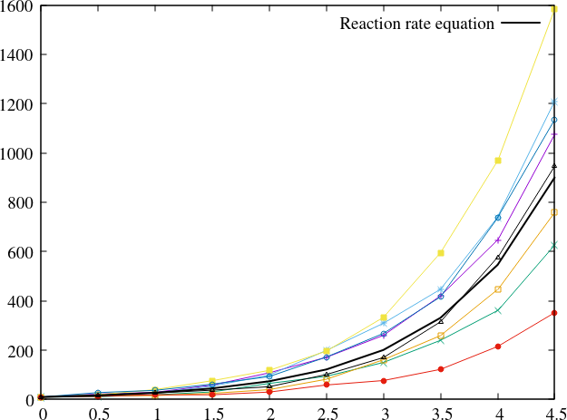
../_images/KineticMonteCarloC1.png — Fig. 23 Comparison of Kinetic Monte Carlo solution with reaction rate equation for an avalanche-like problem.

C2: Schlögl model

Solution the Schlögl model are given in $DISCHARGE_HOME/Exec/Convergence/KineticMonteCarlo/C2. For the Schlögl model we solve for a single population $X$ with the reactions

\[\begin{split}B_1 + 2X &\xrightarrow{c_1} 3X, \\ 3X &\xrightarrow{c_2} B1 + 2X, \\ B2 &\xrightarrow{c_3} X, \\ X &\xrightarrow{c_4} B2.\end{split}\]

The states $B_1$ and $B_2$ are buffered states with populations that do not change during the reactions. Figure Fig. 23 shows the Kinetic Monte Carlo solutions for rates

\[\begin{split}c_1 &= 3\times 10^{-7}, \\ c_2 &= 10^{-4}, \\ c_3 &= 10^{-3}, \\ c_4 &= 3.5\end{split}\]

and $B_1 = 10^5$, $B_2 = 2\times 10^5$. The initial state is $X(0) = 250$.

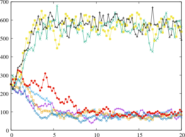
../_images/KineticMonteCarloC2.png — Fig. 24 Convergence to bi-stable states for the Schlögl model.