Advection-diffusion model

The advection-diffusion model simply advects a scalar quantity with EB and AMR. The equation of motion is

\[\frac{\partial\phi}{\partial t} + \nabla\cdot\left(\mathbf{v}\phi - D\nabla\phi\right) = 0.\]

The full implementation for this model consists of the following classes:

AdvectionDiffusionStepper, which implements TimeStepper.
AdvectionDiffusionSpecies, which parses the initial conditions into the problem.
AdvectionDiffusionTagger, which implements CellTagger and flags cells for refinement and coarsening.

The source code for this problem is found in $DISCHARGE_HOME/Physics/AdvectionDiffusion. See AdvectionDiffusionStepper for the C++ API for this time stepper.

Solvers

This class uses the following solvers:

CdrSolver.

Time stepping

Two time stepping algorithms are supported:

A second-order Runge-Kutta method (Heun’s method).
An implicit-explicit method (IMEX) which uses corner-transport upwind (CTU, see CdrCTU) and a Crank-Nicholson diffusion solve.

To select an integrator, set

AdvectionDiffusion.integrator = imex # 'imex' or 'heun'

The user can set the CFL number and maximum/minimum permitted time steps by

AdvectionDiffusion.cfl    = 0.5
AdvectionDiffusion.min_dt = 0.0
AdvectionDiffusion.max_dt = 1.E99

where AdvectionDiffusion.cfl is computed differently based on the chosen discretization.

Heun’s method

For Heun’s method we perform the following steps: Let $\left[\nabla\cdot\mathbf{J}\left(\phi\right)\right]$ be the finite-volume approximation to $\nabla\cdot\left(\mathbf{v}\phi - D\nabla\phi\right)$, where $\mathbf{J}\left(\phi\right) = \mathbf{v}\phi - D\nabla\phi$. The Runge-Kutta advance is then

\[\begin{split}\phi^\prime &= \phi^k - \Delta t\left[\nabla\cdot\mathbf{J}\left(\phi^k\right)\right]\\ \phi^{k+1} &= \phi^k - \frac{\Delta t}{2}\left(\left[\nabla\cdot\mathbf{J}\left(\phi^k\right)\right] + \left[\nabla\cdot\mathbf{J}\left(\phi^\prime\right)\right]\right)\end{split}\]

Note that when diffusion and advecting is coupled in this way, we do not include the transverse terms in the CTU discretization and limit the time step by

\[\Delta t \leq \frac{1}{\frac{\sum_{i=1}^d |v_i|}{\Delta x} + \frac{2dD}{\Delta x^2}},\]

where $d$ is the dimensionality and $D$ is the diffusion coefficient.

IMEX

For the implicit-explicit advance, we use the CTU discretization to center the divergence at the half time step. We seek the update

\[\frac{\phi^{k+1} - \phi^k}{\Delta t} - \frac{1}{2}\left[\nabla\left(D\nabla\phi^k\right) + \nabla\left(D\nabla\phi^{k+1}\right)\right] = -\nabla\cdot\mathbf{v}\phi^{k+1/2},\]

which is a Crank-Nicholson discretization of the diffusion equation with a source term centered on $k+1/2$. We use the CTU discretization (see CdrCTU) for computing the edge states $\phi^{k+1/2}$ and then complete the update by solving the corresponding Helmholtz equation

\[\phi^{k+1} - \frac{\Delta t}{2}\nabla\left(D\nabla\phi^{k+1}\right) = \phi^k - \Delta t\nabla\cdot\mathbf{v}\phi^{k+1/2} + \frac{\Delta t}{2}\nabla\left(D\nabla\phi^k\right)\]

In this case the time step limitation is

\[\Delta t \leq \frac{\Delta x}{\sum_i^d\left|v_i\right|}.\]

Warning

It is possible to use this module with any implementation of CdrSolver, but the IMEX discretization only makes sense if the hyperbolic term can be centered on $k+1/2$.

If the truncation order of $\phi^{k+1/2}$ is $\mathcal{O}\left(\Delta t^2\right)$, the resulting IMEX discretization is globally second order accurate. For the CdrCTU discretization the edge states are accurate to $\mathcal{O}\left(\Delta t\Delta x\right)$, so the scheme is globally first order convergent (but with a small error constant).

Initial data

Default behavior

By default, the initial data for this problem is given by a super-Gaussian blob

\[\phi\left(\mathbf{x},t=0\right) = \phi_0\exp\left(-\frac{\left|\mathbf{x}-\mathbf{x}_0\right|^4}{2R^4}\right),\]

where $\phi_0$ is an amplitude, $\mathbf{x}_0$ is the blob center and $R$ is the blob radius. These are set by the input options

AdvectionDiffusion.blob_amplitude = 1.0
AdvectionDiffusion.blob_radius    = 0.1
AdvectionDiffusion.blob_center    = 0 0 0

Custom value

For a more general way of specifying initial data, AdvectionDiffusionStepper has a public member function

void setInitialData(const std::function<Real(const RealVect& a_pos)>& a_func) noexcept;

Velocity field

Default behavior

The default velocity field for this class is

\[\begin{split}v_x &= -r\omega\sin\theta, \\ v_y &= r\omega\cos\theta, \\ v_z &= 0,\end{split}\]

where $r = \sqrt{x^2 + y^2}$, $\tan\theta = \frac{x}{y}$. I.e. the flow field is a circulation around the Cartesian grid origin.

To adjust the velocity field through $\omega$, set

AdvectionDiffusion.omega  = 1.0

Custom value

For a more general way of setting a user-specified velocity, AdvectionDiffusionStepper has a public member function

void setVelocity(const std::function<RealVect(const RealVect a_position)>& a_velocity) noexcept;

Diffusion coefficient

Default behavior

The default diffusion coefficient for this problem is set to a constant. To adjust it, $\omega$, set

AdvectionDiffusion.diffco = 1.0

to a chosen value.

Custom value

For a more general way of setting the diffusion coefficient, AdvectionDiffusionStepper has a public member function

void setDiffusionCoefficient(const std::function<Real(const RealVect a_position)>& a_diffusion) noexcept;

Boundary conditions

At the EB, this module uses a wall boundary condition (i.e. no flux into or out of the EB). On domain edges (faces in 3D), the user can select between wall boundary conditions or outflow boundary conditions by selecting the corresponding input option for the solver. E.g. for the CdrCTU discretization:

CdrCTU.bc.x.lo = wall # 'wall' or 'outflow'
CdrCTU.bc.x.hi = wall # 'wall' or 'outflow'

The syntax for the other boundaries are completely analogous.

Setting up a new problem

To set up a new problem, using the Python setup tools in $DISCHARGE_HOME/Physics/AdvectionDiffusion is the simplest way. To see available setup options, run

./setup.py --help

For example, to set up a new problem in $DISCHARGE_HOME/MyApplications/MyAdvectionDiffusionProblem for a coaxial cable geometry, run

./setup.py -base_dir=MyApplications -app_name=MyAdvectionDiffusionProblem -geometry=CoaxialCable

This will set up a new problem in a coaxial cable geometry (defined in Geometries/CoaxialCable).

Example programs

Some example programs for this module are given in

$DISCHARGE_HOME/Exec/Examples/AdvectionDiffusion/DiagonalFlowNoEB
$DISCHARGE_HOME/Exec/Examples/AdvectionDiffusion/PipeFlow

Verification

Spatial and temporal convergence tests for this module (and thus also the underlying solver implementation) are given in

$DISCHARGE_HOME/Exec/Convergence/AdvectionDiffusion/C1
$DISCHARGE_HOME/Exec/Convergence/AdvectionDiffusion/C2

C1: Spatial convergence

A spatial convergence test is given in $DISCHARGE_HOME/Exec/Convergence/AdvectionDiffusion/C1. The problem solves for an advected and diffused scalar in a rotational velocity in the presence of an EB:

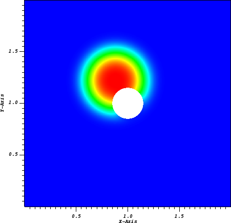
../_images/AdvectionDiffusionC1_1.png — Fig. 25 Final state on a $512^2$ uniform grid.

To compute the convergence rate we compute two solutions with grid spacings $\Delta x$ and $\Delta x/2$, and estimate the solution error using the approach in Spatial convergence. Figure Fig. 26 shows the computed convergence rates with various choice of slope limiters. We find 2nd order convergence in all three norms for sufficiently fine grid when using slope limiters, and first order convergence when limiters are turned off. The reduced convergence rates at coarser grids occur due to 1) insufficient resolution of the initial density profile and 2) under-resolution of the geometry.

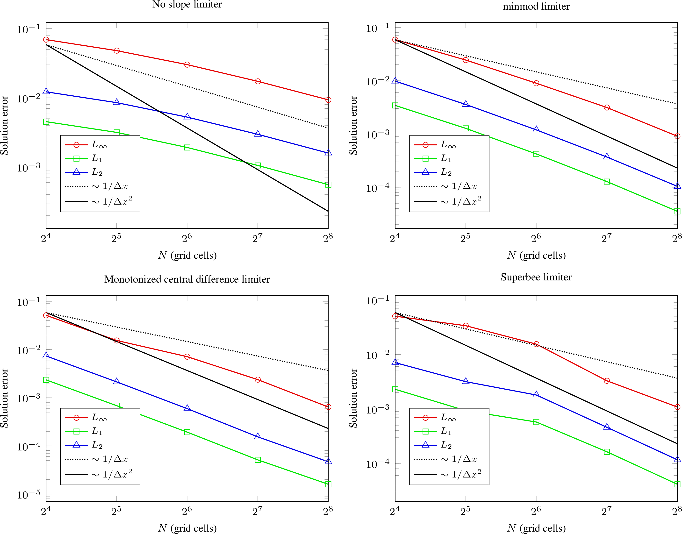
../_images/AdvectionDiffusionC1_2.png — Fig. 26 Spatial convergence rates with various limiters.

C2: Temporal convergence

A temporal convergence test is given in $DISCHARGE_HOME/Exec/Convergence/AdvectionDiffusion/C2. To compute the temporal convergence rate we compute two solutions using time steps $\Delta t$ and $\Delta t/2$, and estimate the solution error using the approach in Temporal convergence. Figure Fig. 27 shows the computed convergence rates for the second order Runge-Kutta and the IMEX discretization. As expected, we find 2nd order convergence for Heun’s method and first order convergence for the IMEX discretization.

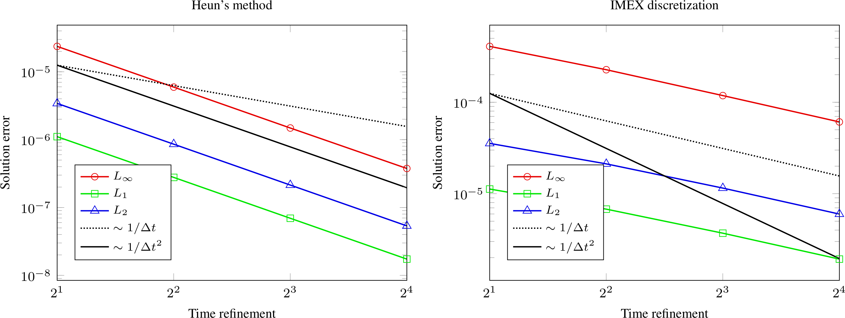
../_images/AdvectionDiffusionC2.png — Fig. 27 Temporal convergence rates.

Advection-diffusion model

Solvers

Time stepping

Heun’s method

IMEX

Initial data

Default behavior

Custom value

Velocity field

Default behavior

Custom value

Diffusion coefficient

Default behavior

Custom value

Boundary conditions

Cell refinement

Setting up a new problem

Example programs

Verification

C1: Spatial convergence

C2: Temporal convergence