Spatial discretization
Cartesian AMR
chombo-discharge uses Cartesian patch-based structured adaptive mesh refinement (AMR) provided by Chombo [Colella et al., 2004].
In patch-based AMR the domain is subdivided into a collection of hierarchically nested grid levels, see Fig. 2, where each grid level consist of a set of rectangular grid blocks.
I.e., a grid level is composed of a union of grid patches sharing the same grid resolution, with the additional requirement that the patches on a grid level are non-overlapping.
With AMR, such levels can be hierarchically nested; finer grid levels exist on top of coarser ones.
In patch-based AMR there are only a few fundamental requirements on how such grids are constructed.
For example, a refined grid level must exist completely within its parent (i.e., coarser) grid.
In other words, grid levels \(l-1\) and \(l+1\) are spatially separated by a non-zero number of grid cells on level \(l\).
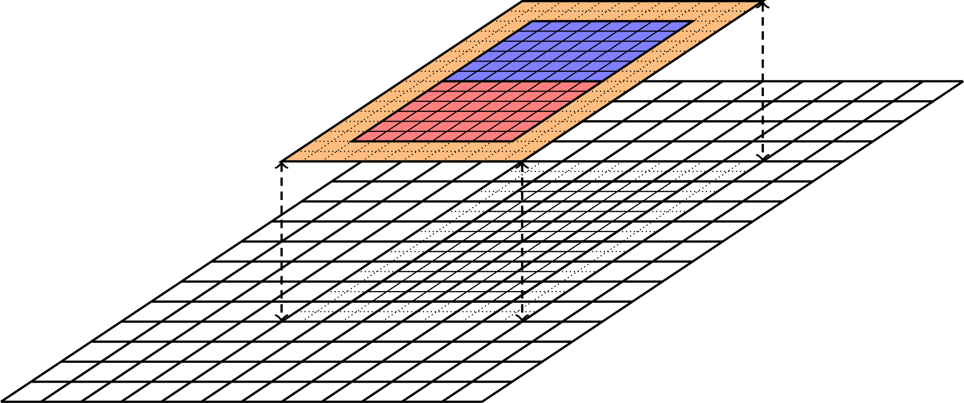
Fig. 2 Cartesian patch-based refinement showing two grid levels. The fine-grid level lives on top of the coarse level, and consists of two patches (red and blue colors) with two layers of ghost cells (dashed lines and orange shaded region).
The resolution on level \(l+1\) is typically finer than the resolution on level \(l\) by an integer (usually power of two).
Important
chombo-discharge only supports refinement factors of 2 and 4, with a few limitations for factor 4 refinement.
Embedded boundaries
chombo-discharges uses an embedded boundary (EB) formulation for describing complex geometries.
With EBs, the Cartesian grid is directly intersected by the geometry.
This is fundamentally different from unstructured grid where one generates a volume mesh that conforms to the surface mesh of the input geometry.
Since EBs are directly intersected by the geometry, there is no fundamental need for a surface mesh for describing the geometry.
Moreover, Cartesian EBs have a data layout which remains (almost) fully structured.
The connectivity of neighboring grid cells is still trivially found by fundamental strides along the data rows/columns, which allows extending the efficiency of patch-based AMR to complex geometries.
Fig. 3 shows an example of patch-based grid refinement for a complex surface.
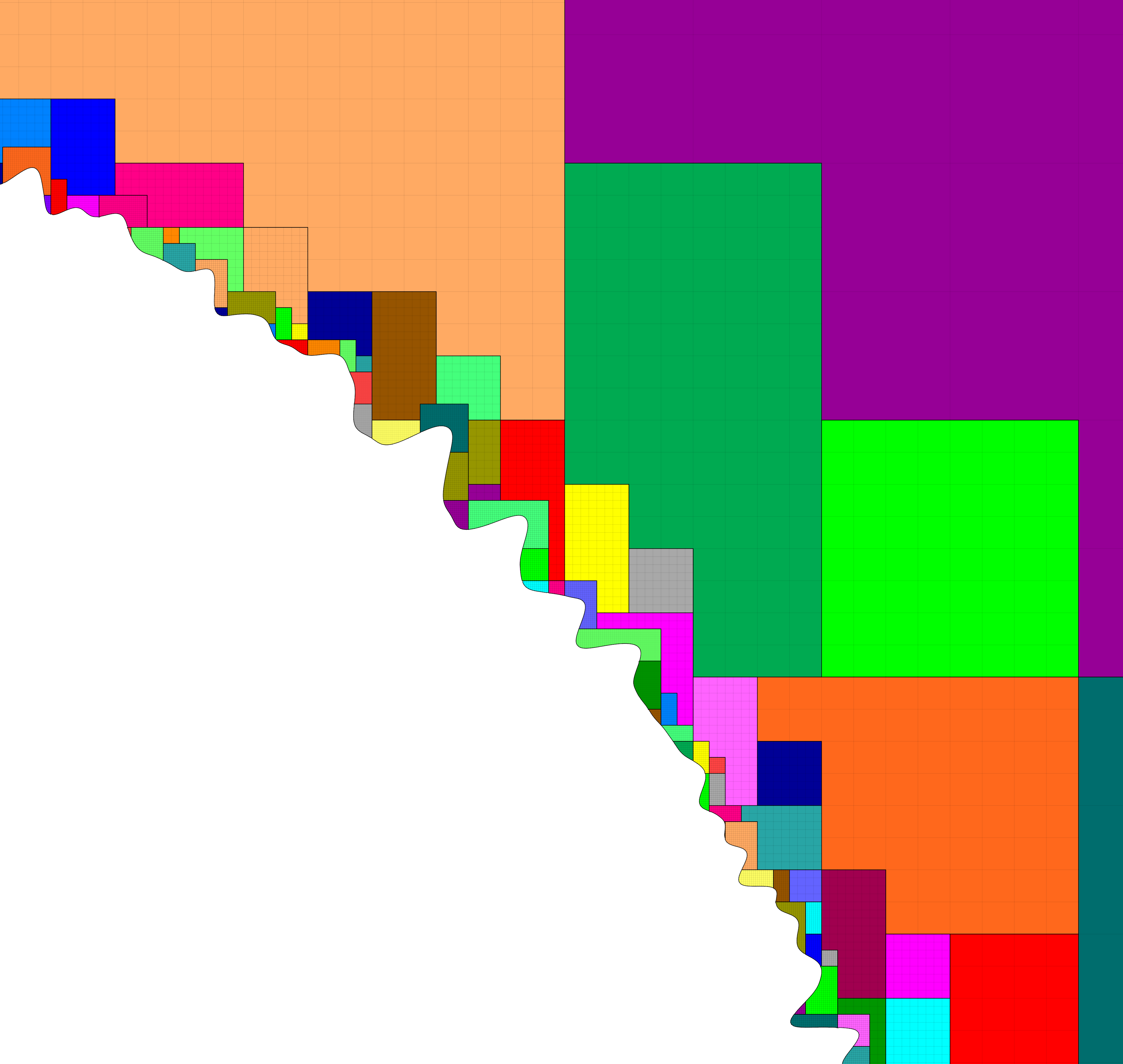
Fig. 3 Patch-based refinement (factor 4 between levels) of a complex surface. Each color shows a patch, which is a rectangular computational unit.
Since EBs are directly intersected by the geometry, pathological cases can arise where coarsening of a grid cell leads to a coarser cell consisting of multiple volumes. One can easily envision this case by intersecting a thin body with a Cartesian grid, as shown in Fig. 4. This figure shows a thin body which is intersected by a Cartesian grid, and this grid is then coarsened. At the coarsened level, one of the grid cells has two cell fragments on opposite sides of the body. Such multi-valued cells (a.k.a multi-cells) are fundamentally important for EB applications when coarsening is involved. Note that there is no fundamental difference between single-cut and multi-cut grid cells. This distinction exists primarily due to the fact that if all grid cells were single-cut cells the entire EB data structure would fit in a Cartesian grid block (say, of \(N_x \times N_y \times N_z\) grid cells). However, because of multi-cells, EB data structures are not purely Cartesian. Data structures need to live on more complex graphs that describe the multi-cells and, furthermore, describe the cell connectivity between cut-cell volumes. Without multi-cells it would be impossible to describe most complex geometries, and it is extremely difficult to obtain performant geometric multigrid methods which instrinsically rely on this type of coarsening.
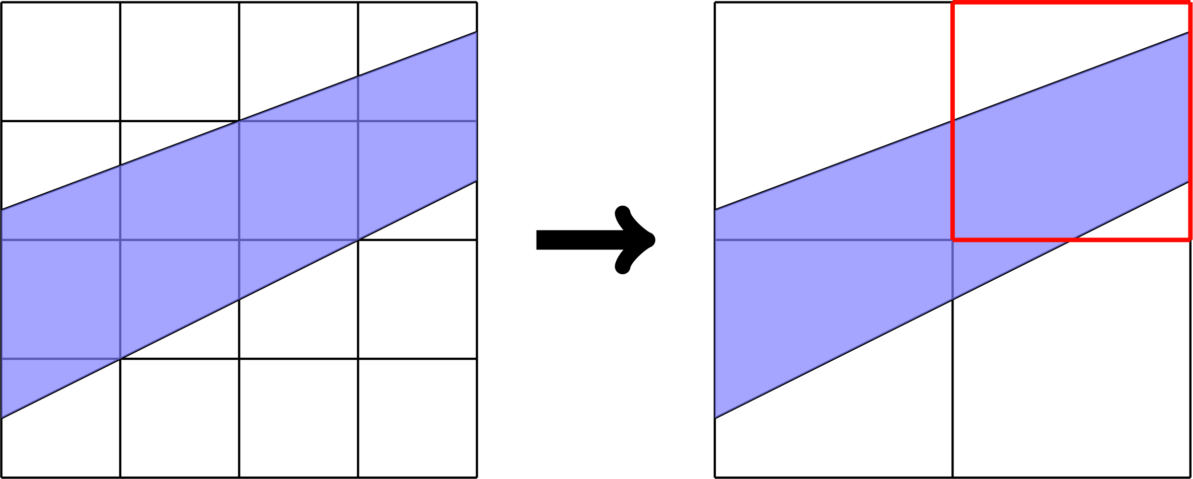
Fig. 4 Example of how multi-valued cells occur during grid coarsening. Left: Original grid. Right: Coarsened grid where one grid cell is multi-valued.
Geometry representation
chombo-discharge uses (approximations to) signed distance functions (SDFs) for describing geometries.
Signed distance fields are functions \(f: \mathbb{R}^3\rightarrow \mathbb{R}\) that describe the distance from the object.
These functions are also implicit functions, i.e., \(f\left(\mathbf{x}\right)=0\) describes the surface of the object, \(f\left(\mathbf{x}\right) > 0\) describes a point inside the object and \(f\left(\mathbf{x}\right) < 0\) describes a point outside the object.
Many EB applications only use the implicit function formulation, but chombo-discharge requires (an approximation to) the signed distance field for the following reasons:
There are two reasons for this:
The SDF can be used for robustly load balancing the geometry generation with orders of magnitude speedup over naive approaches.
The SDF is useful for resolving particle collisions with boundaries, and permit mesh-less ray-tracing of computational particles.
To illustrate the difference between an SDF and an implicit function, consider the implicit functions for a sphere at the origin with radius \(R\):
Here, only \(d_1\left(\mathbf{x}\right)\) is a signed distance function.
In chombo-discharge, SDFs can be generated through analytic expressions, constructive solid geometry, or by supplying polygon tessellation.
NURBS geometries are not supported.
Fundamentally, all geometric objects are described using BaseIF objects from Chombo, see BaseIF.
Constructive solid geometry (CSG)
Constructive solid geometry can be used to generate complex shapes from geometric primitives. For example, to describe the union between two SDFs \(d_1\left(\mathbf{x}\right)\) and \(d_2\left(\mathbf{x}\right)\):
Note that the resulting is an implicit function but is not an SDF.
However, the union typically approximates the signed distance field quite well near the surface.
Chombo natively supports many ways of performing CSG.
EBGeometry
While functions like \(R - \left|\mathbf{x}\right|\) are quick to compute, a polygon surface may consist of hundreds of thousands of primitives (e.g., triangles).
Generating signed distance function from polygon tessellations is quite involved as it requires computing the signed distance to the closest feature, which can be a planar polygon (e.g., a triangle), edge, or a vertex.
chombo-discharge supports such functions through the EBGeometry package.
Warning
The signed distance function for a polygon surface is only well-defined if it is manifold-2, i.e., it is watertight and does not self-intersect.
Searching through all features (faces, edge, vertices) is unacceptably slow, and EBGeometry therefore uses a bounding volume hierarchy for accelerating these searches.
The bounding volume hierarchy is top-down constructed, using a root bounding volume (typically a cube) that encloses all triangles.
Using heuristics, the root bounding volume is then subdivided into two separate bounding volumes that contain roughly half of the primitives each.
The process is then recursed downwards until specified recursion criteria are met.
Additional details are provided in the EBGeometry documentation.
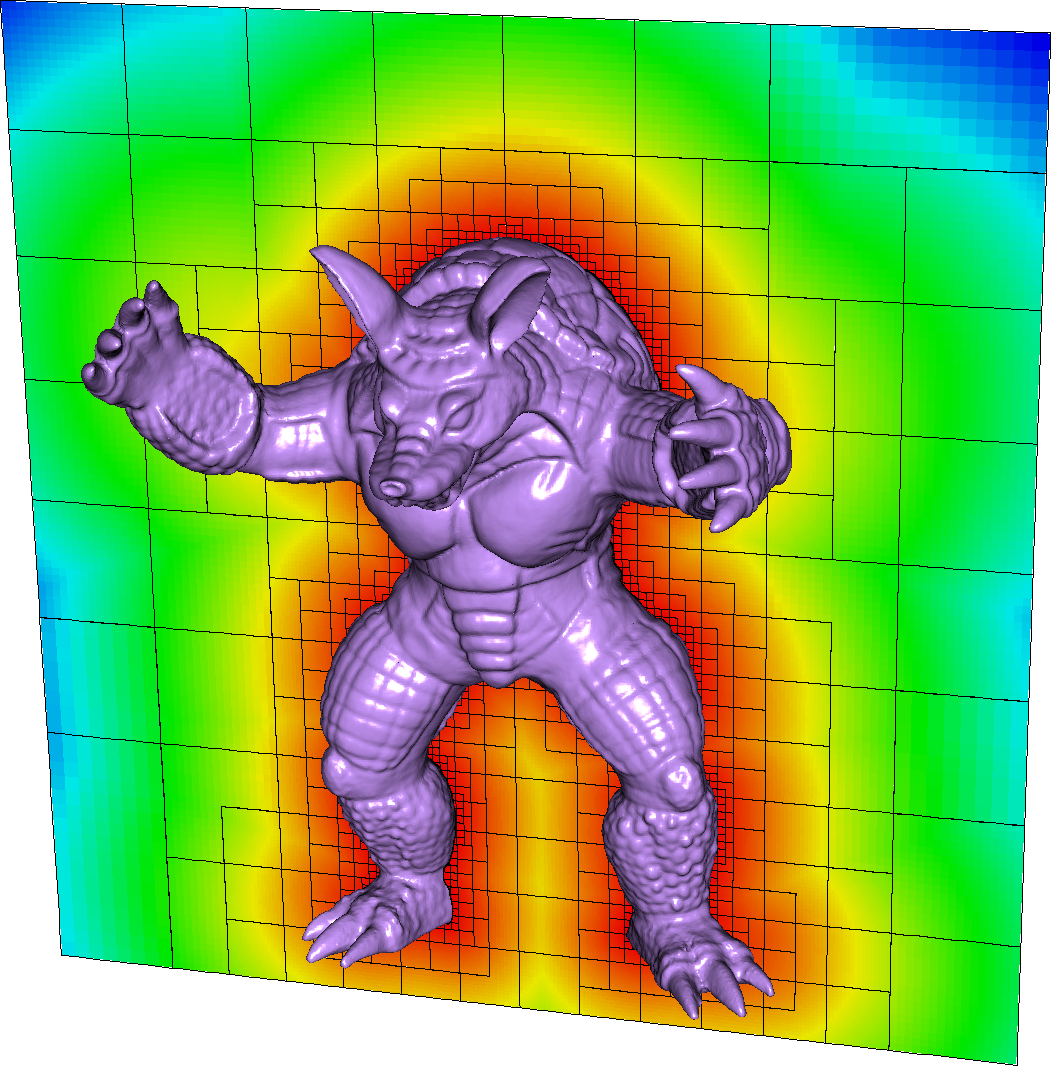
Fig. 5 Example of an SDF reconstruction and cut-cell grid from a surface tessellation in chombo-discharge.
Geometry generation
Chombo approach
The default geometry generation method in Chombo is to locate cut-cells on the finest AMR level first and then generate the coarser levels cells through grid coarsening.
This will look through all cells on the finest level, so for a domain which is effectively \(N\times N\times N\) cells there are \(\mathcal{O}\left(N^3\right)\) implicit function queries.
In 2D, the complexity is \(\mathcal{O}\left(N^2\right)\).
However, as \(N\) becomes large, say \(N=10^5\), geometric queries of this type quickly become a bottleneck and the algorithm becomes practically unusable.
chombo-discharge pruning
chombo-discharge has made modifications to the geometry generation routines in Chombo, resolving a few bugs and, most importantly, using the signed distance function for load balancing the geometry generation step.
This modification to Chombo yields a reduction of the original \(\mathcal{O}\left(N^3\right)\) scaling in Chombo grid generation to an \(\mathcal{O}\left(N^2\right)\) scaling in chombo-discharge.
Typically, we find that this makes geometry generation computationally trivial for geometries consisting of relatively small object surface areas.
To understand this process, note that the SDF satisfies the Eikonal equation
and so it is well-behaved for all \(\mathbf{x}\). The SDF can thus be used to prune large regions in space where cut-cells don’t exist. For example, consider a Cartesian grid patch with cell size \(\Delta x\) and cell-centered grid points \(\mathbf{x}_{\mathbf{i}} = \left(\mathbf{i} + \mathbf{\frac{1}{2}}\right)\Delta x\) where \(\mathbf{i} \in \mathbb{Z}^3\) are grid cells in the patch, as shown in Fig. 6. We know that cut cells do not exist in the grid patch if \(\left|f\left(\mathbf{x}_{\mathbf{i}}\right)\right| > \frac{\sqrt{3}\Delta x}{2}\) for all \(\mathbf{i}\) in the patch. One can use this to perform a quick scan of the SDF on a coarse grid level first, for example on \(l=0\), and recurse deeper into the grid hierarchy to locate cut-cells on the other levels. Typically, a level is decomposed into Cartesian subregions, and each subregion can be scanned independently of the other subregions, so the problem lends itself naturally to parallelization. By default, partitioning of subregions is done using a Morton curve. Subregions that can’t contain cut-cells are designated as inside or outside, depending on the sign of the SDF. There is no point in recursively refining these to look for cut-cells at finer grid levels, owing to the nature of the SDF they can be safely pruned from subsequent scans at finer levels. The subregions that did contain cut-cells are refined and decomposed into sub-subregions. This procedure recurses until \(l=l_{\text{max}}\), at which point we have determined all sub-regions in space where cut-cells can exist (on each AMR level), and pruned the ones that don’t. This process is shown in Fig. 6. Once all the grid patches that contain cut-cells have been found, these patches are distributed (i.e., load balanced) to the various MPI ranks for computing the discrete grid information.
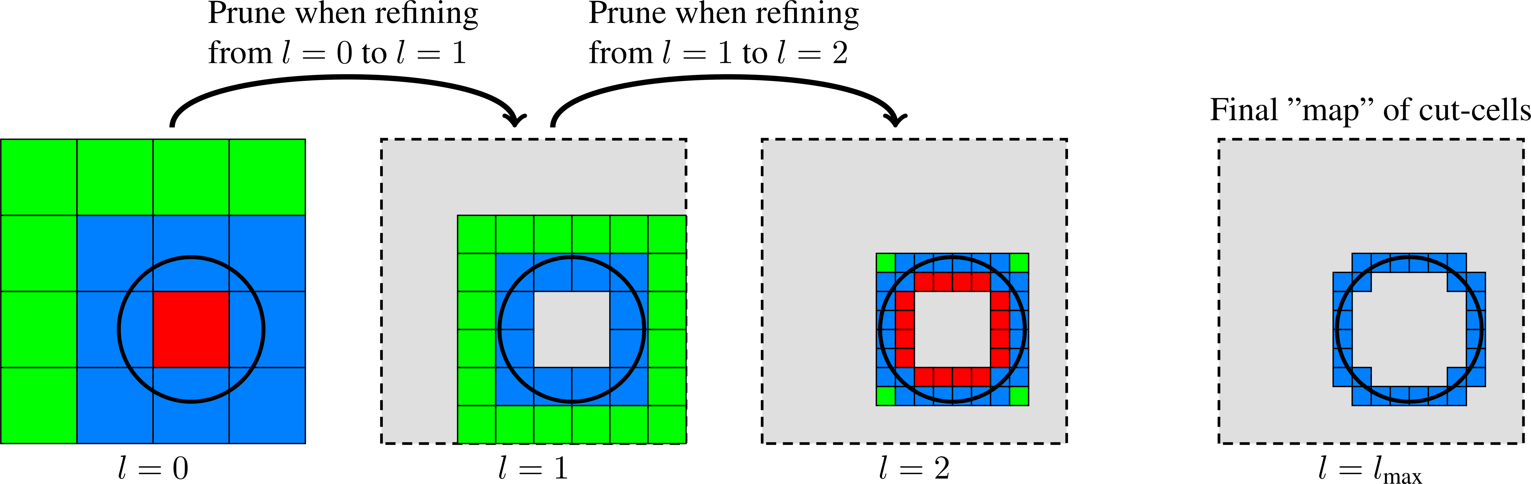
Fig. 6 Pruning cut-cells with the signed distance field. Red-colored grid patches are grid patches entirely contained inside the EB. Green-colored grid patches are entirely outside the EB, while blue-colored grid patches contain cut-cells.
The above load balancing strategy is very simple, and it reduces the original \(O(N^3)\) complexity in 3D to \(O(N^2)\) complexity, while in 2D the complexity is reduced from \(O(N^2)\) to \(O(N)\). The strategy works for all SDFs although, strictly speaking, an SDF is not fundamentally needed. If a well-behaved Taylor series can be found for an implicit function, the bounds on the series can also be used to infer the location of the cut-cells, and the same algorithm can be used. For example, generating compound objects with CSG are typically sufficiently well behaved (provided that the components are SDFs). However, implicit functions like \(d\left(\mathbf{x}\right) = R^2 - \mathbf{x}\cdot\mathbf{x}\) must be used with caution.
Mesh generation
chombo-discharge supports two grid generation algorithms:
The classical Berger-Rigoutsos algorithm [Berger and Rigoutsos, 1991].
A tiled algorithm [Gunney and Anderson, 2016].
Both algorithms work by taking a set of flagged cells on each grid level and generating new boxes that cover the flags. Only properly nested grids are generated, in which case two grid levels \(l-1\) and \(l+1\) are separated by a non-zero number of grid cells on level \(l\). This requirement is not fundamentally required for quadtree and octree grids, but is nevertheless usually imposed. For patch based AMR, the rationale for this requirement is that stencils on level \(l+1\) should should only reach into grid cells on levels \(l\) and \(l+1\), which greatly simplifies the definition of numerical stencils on each level. For example, ghost cells on level \(l+1\) can then be interpolated from data only on levels \(l\) and \(l+1\).
Berger-Rigoutsos algorithm
The Berger-Rigoustous grid algorithm is implemented in Chombo and can be called by chombo-discharge.
The classical Berger-Rigoustous algorithm is inherently serial in the sense that is collects the flagged cells onto each MPI rank and then generates the boxes, see [Berger and Rigoutsos, 1991] for implementation details.
Typically, it is not used at large scale in 3D due to its memory consumption.
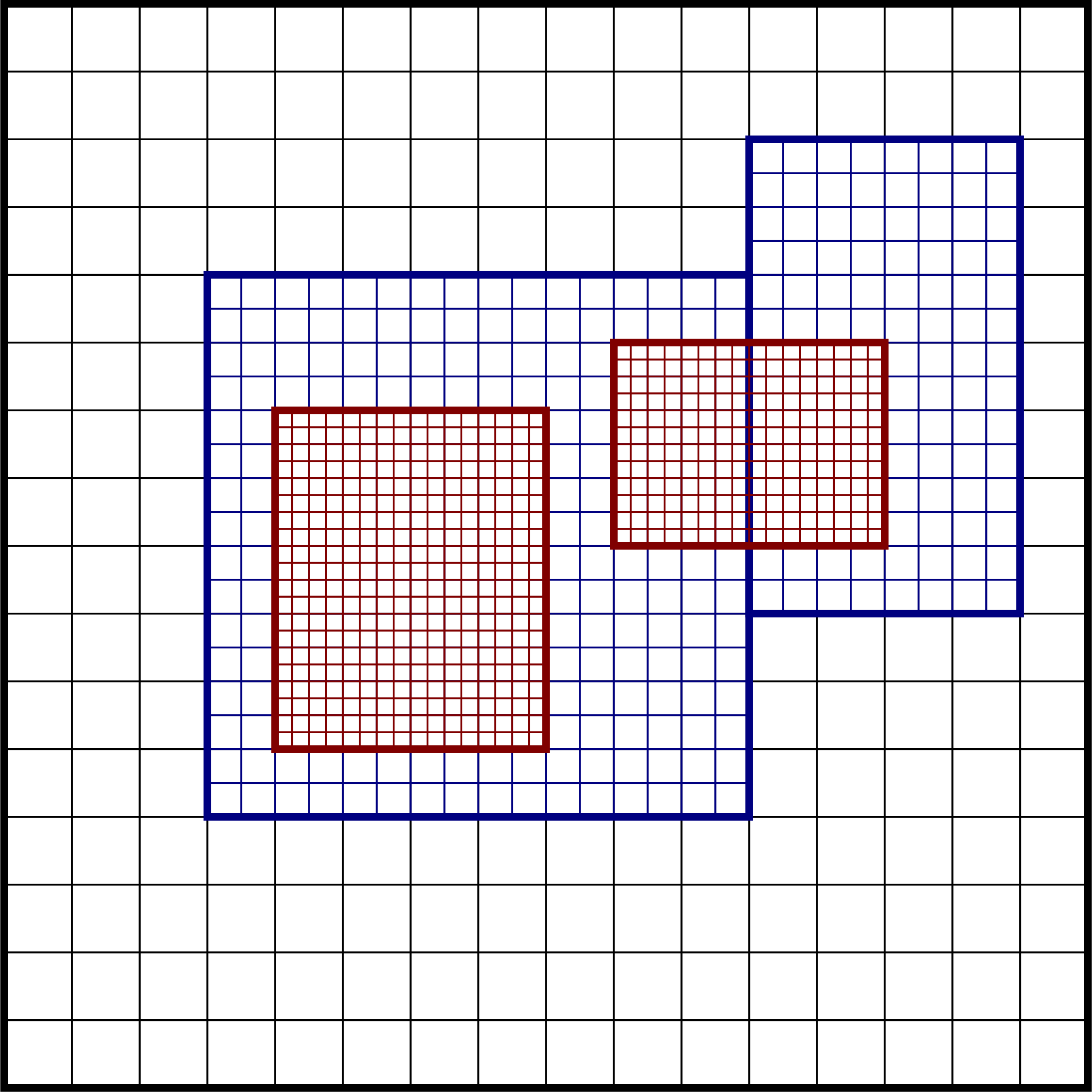
Fig. 7 Classical cartoon of patch-based refinement. Bold lines indicate entire grid blocks.
Tiled mesh refinement
chombo-discharge also supports a tiled algorithm where the grid boxes on each block are generated according to a predefined tiled pattern.
If a tile contains a single tag, the entire tile is flagged for refinement.
The tiled algorithm produces grids that are visually similar to octrees, but is slightly more general since it also supports refinement factors other than 2 and is not restricted to domain extensions that are an integer factor of 2 (e.g. \(2^{10}\) cells in each direction).
Moreover, the algorithm is extremely fast and has low memory consumption even at large scales.
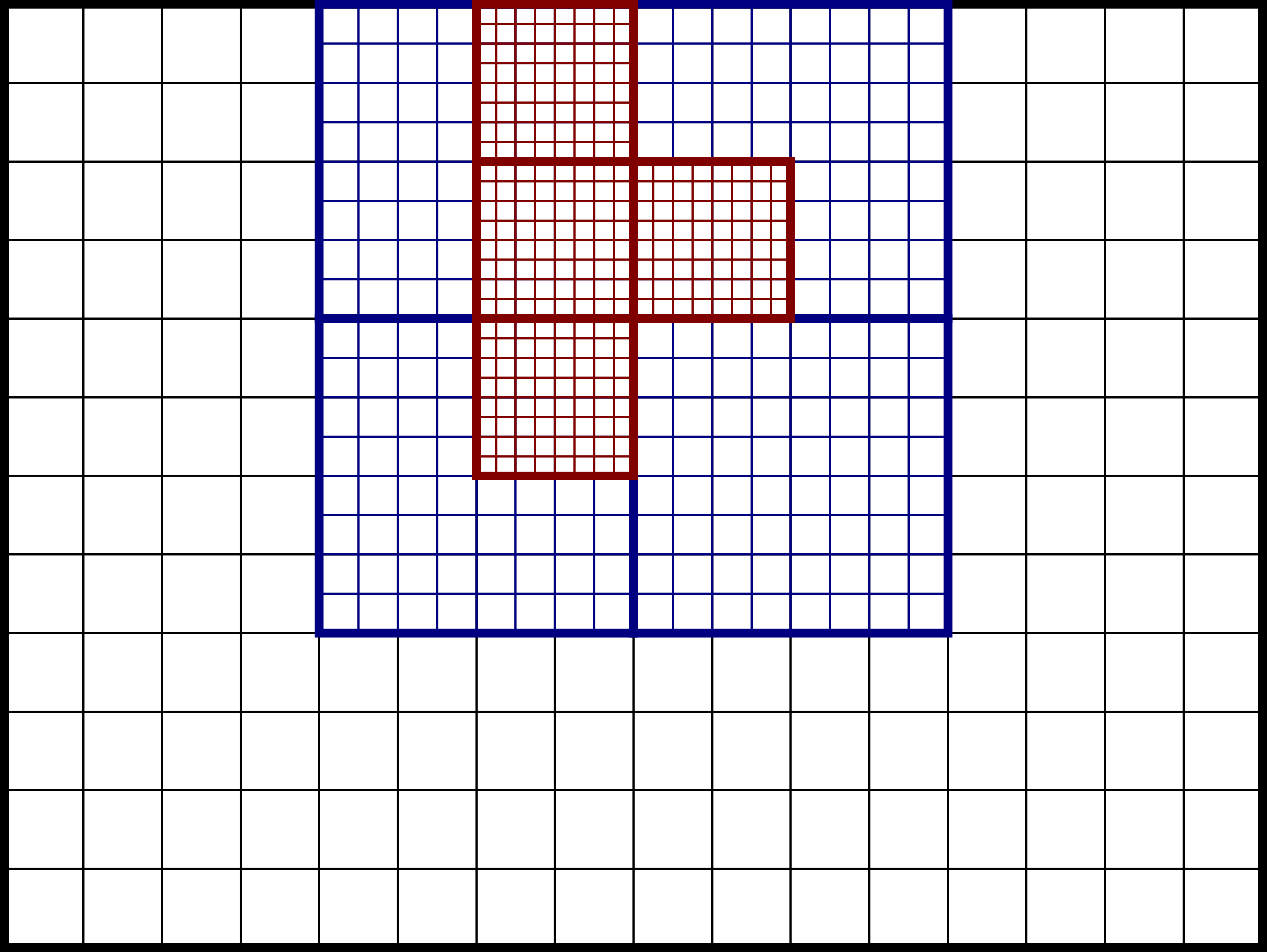
Fig. 8 Classical cartoon of tiled patch-based refinement. Bold lines indicate entire grid blocks.
Cell refinement philosophy
chombo-discharge can flag cells for refinement using various methods:
Refine all embedded boundaries down to a specified refinement level. See Driver.
Refine embedded boundaries based on estimations of the surface curvature in the cut-cells. See Driver.
Manually add refinement flags (by specifying boxes where cells will be refined). See CellTagger.
Physics-based or data-based refinement where the user fetches data from solver classes (e.g., discretization errors, the electric field) and uses that for refinement. See CellTagger.
The first two cases are covered by the Driver class in chombo-discharge.
In the first case Driver will simply fetch arguments from an input script which specifies the refinement depth for the embedded boundaries.
In the second case, the Driver class will visit every cut-cell and check if the normal vectors in neighboring cut-cell deviate by more than a specified threshold angle.
Given two normal vectors \(\mathbf{n}\) and \(\mathbf{n}^\prime\), the cell is refined if
where \(\theta_c\) is a threshold angle for grid refinent.
The other two cases are more complicated, and are covered by the CellTagger classes.