Convection-Diffusion-Reaction
Here, we discuss the discretization of the equation
We assume that \(\phi\) is discretized by cell-centered averages (note that cell centers may lie inside solid boundaries), and use finite volume methods to construct fluxes in a cut-cells and regular cells. Here, \(\mathbf{v}\) indicates a drift velocity and \(D\) is the (isotropic) diffusion coefficient.
Note
Using cell-centered versions \(\phi\) might be problematic for some models since the state is extended outside the valid region. Models might have to recenter the state in order compute e.g. physically meaningful reaction terms in cut-cells.
Tip
Source code for the convection-diffusion-reaction solvers reside in $DISCHARGE_HOME/Source/ConvectionDiffusionReaction.
CdrSolver
The CdrSolver class contains the interface for solving advection-diffusion-reaction problems.
CdrSolver is an abstract class and does not contain any specific advective or diffusive discretization (these are added by implementation classes).
However, CdrSolver supplies a useful interface that includes implementations of regrid functions and I/O capabilities, such that only the advective and diffusive discretizations need to be provided.
The implementation layers of the CDR capabilities consist of the following:
CdrMultigrid, which inherits from
CdrSolverand adds a second order accurate discretization for the diffusion operator. This includes both explicit and implicit discretizations, where the implicit discretization uses geometric multigrid to resolve the diffusion problem.CdrCTU and CdrGodunov which inherit from
CdrMultigridand add a second order accurate spatial discretization for the advection operator.
Currently, we mostly use the CdrCTU class which contains a second order accurate discretization with slope limiters.
CdrGodunov is a similar operator, but the advection code for this is distributed by the Chombo team.
The C++ API for these classes can be obtained from https://chombo-discharge.github.io/chombo-discharge/doxygen/html/classCdrSolver.html and references therein.
Explicit advance methods for Eq. 5 only require an approximation to the right-hand side of the equation. These approximations are encapsulated by the following functions:
/**
  @brief Compute div(J) explicitly, where J = nV - D*grad(n)
  @param[out] a_divJ             Divergence term, i.e. finite volume approximation to
  @param[in]  a_phi              Cell-centered state
  @param[in]  a_extrapDt         Extrapolation in time, i.e. shifting of div(J) towards e.g. half time step. Only affects the advective term.
  @param[in]  a_conservativeOnly If true, we compute div(J) = 1/dx*sum(fluxes), which does not involve redistribution.
  @param[in]  a_ebFlux           If true, the embedded boundary flux will injected and included in div(J)
  @param[in]  a_domainFlux       If true, the domain flux will injected and included in div(J)
  @note a_phi is non-const because ghost cells will be re-filled
*/
virtual void
computeDivJ(EBAMRCellData& a_divJ,
            EBAMRCellData& a_phi,
            const Real     a_extrapDt,
            const bool     a_conservativeOnly,
            const bool     a_ebFlux,
            const bool     a_domainFlux) = 0;

/**
  @brief Compute div(v*phi) explicitly
  @param[out] a_divF             Divergence term, i.e. finite volume approximation to Div(v*phi), including redistribution magic.
  @param[in]  a_phi              Cell-centered state
  @param[in]  a_extrapDt         Extrapolation in time, i.e. shifting of div(F) towards e.g. half time step. Only affects the advective term.
  @param[in]  a_conservativeOnly If true, we compute div(F)=1/dx*sum(fluxes), which does not involve redistribution.
  @param[in]  a_ebFlux           If true, the embedded boundary flux will injected be included in div(F)
  @param[in]  a_domainFlux       If true, the domain flux will injected and included in div(F)
  @note a_phi is non-const because ghost cells will be interpolated in this routine. Valid data in a_phi is not touched.
*/
virtual void
computeDivF(EBAMRCellData& a_divF,
            EBAMRCellData& a_phi,
            const Real     a_extrapDt,
            const bool     a_conservativeOnly,
            const bool     a_ebFlux,
            const bool     a_domainFlux) = 0;

/**
  @brief Compute div(D*grad(phi)) explicitly
  @param[in]  a_phi              Cell-centered state
  @param[in]  a_conservativeOnly If true, we compute div(D) = 1/dx*sum(fluxes), which does not involve redistribution.
  @param[in]  a_domainFlux       If true, the domain flux will injected and included in div(D)
  @note a_phi is non-const because ghost cells will be interpolated in this routine. Valid data in a_phi is not touched.
  @param[in] a_divD Div d
  @param[in] a_ebFlux Eb flux
*/
virtual void
computeDivD(EBAMRCellData& a_divD,
            EBAMRCellData& a_phi,
            const bool     a_conservativeOnly,
            const bool     a_ebFlux,
            const bool     a_domainFlux) = 0;
These functions are not implemented in CdrSolver, but in subclasses.
In the current structure, CdrMultigrid supplies the diffusive discretization and CdrCTU supplies the advective discretization.
The implicit advance methods for CdrSolver are encapsulated by the following functions:
/**
  @brief Implicit diffusion Euler advance with source term.
  @param[in,out] a_newPhi Solution at time t + dt
  @param[in]    a_oldPhi Solution at time t
  @param[in]    a_source Source term.
  @param[in]    a_dt     Time step
  @note For purely implicit Euler the source term should be centered at t+dt (otherwise it's an implicit-explicit method)
  @details This solves the implicit diffusion equation equation a_newPhi - a_oldPhi = dt*Laplacian(a_newPhi) + dt*a_source.
*/
virtual void
advanceEuler(EBAMRCellData&       a_newPhi,
             const EBAMRCellData& a_oldPhi,
             const EBAMRCellData& a_source,
             const Real           a_dt) = 0;

/**
  @brief Implicit diffusion Crank-Nicholson advance with source term.
  @param[in,out] a_newPhi Solution at time t + dt
  @param[in]    a_oldPhi Solution at time t
  @param[in]    a_source Source term.
  @param[in]    a_dt     Time step
*/
virtual void
advanceCrankNicholson(EBAMRCellData&       a_newPhi,
                      const EBAMRCellData& a_oldPhi,
                      const EBAMRCellData& a_source,
                      const Real           a_dt) = 0;
Discretization details
Explicit divergences and redistribution
Computing explicit divergences for equations like
is problematic because of the arbitrarily small volume fractions of cut cells. In general, we seek a method-of-lines update \(\phi^{k+1} = \phi^k - \Delta t \left[\nabla\cdot \mathbf{G}^k\right]\) where \(\left[\nabla\cdot\mathbf{G}\right]\) is a stable numerical approximation based on some finite volume approximation.
Pure finite volume methods use
where \(\kappa\) is the volume fraction of a grid cell, \(\textrm{DIM}\) is the spatial dimension and the volume integral is written as discretized surface integral
The sum runs over all cell edges (faces in 3D) of the cell where \(G_f\) is the flux on the edge centroid and \(\alpha_f\) is the edge (face) aperture.
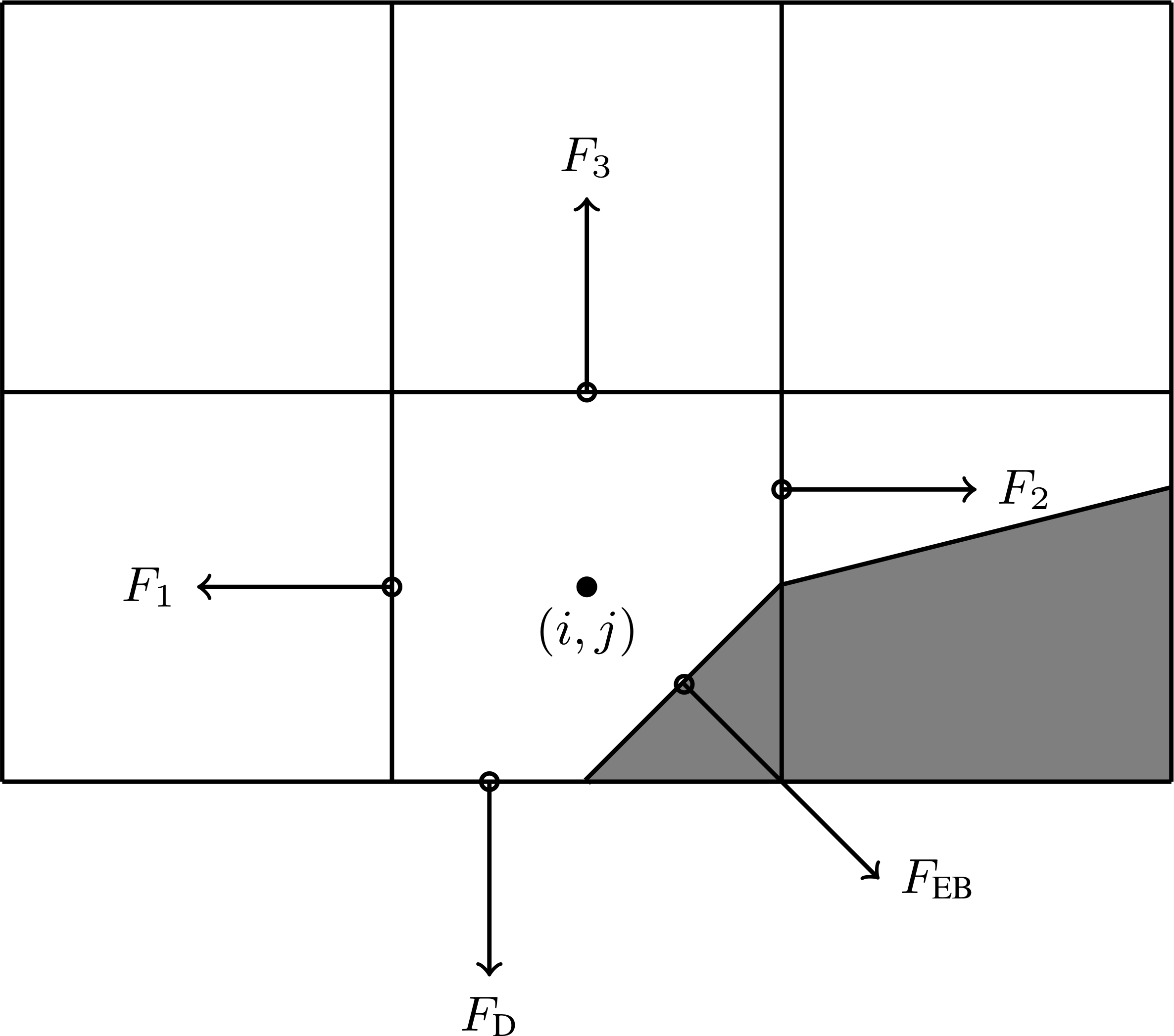
Fig. 22 Location of centroid fluxes for cut cells.
However, taking \([\nabla\cdot\mathbf{G}^k]\) to be this sum leads to a time step constraint proportional to \(\kappa\), which can be arbitrarily small. This leads to an unacceptable time step constraint for Eq. 6. We use the Chombo approach and expand the range of influence of the cut cells in order to stabilize the discretization and allow the use of a normal time step constraint. First, we compute the conservative divergence
where \(G_f = \mathbf{G}_f\cdot \mathbf{n}_f\). Next, we compute a non-conservative divergence \(D_{\mathbf{i}}^{nc}\)
where \(N(\mathbf{i})\) indicates some neighborhood of cells around cell \(\mathbf{i}\). Next, we compute a hybridization of the divergences,
and perform an intermediate update
The hybrid divergence update fails to conserve mass by an amount \(\delta M_{\mathbf{i}} = \kappa_{\mathbf{i}}\left(1-\kappa_{\mathbf{i}}\right)\left(D_{\mathbf{i}}^c - D_{\mathbf{i}}^{nc}\right)\). In order to main overall conservation, the excess mass is redistributed into neighboring grid cells. Let \(\delta M_{\mathbf{i}, \mathbf{j}}\) be the redistributed mass from \(\mathbf{j}\) to \(\mathbf{i}\) where
This mass is used as a local correction in the vicinity of the cut cells, i.e.
where \(\delta M_{\mathbf{j}\in N(\mathbf{i}), \mathbf{i}}\) is the total mass redistributed to cell \(\mathbf{i}\) from the other cells. After these steps, we define
Numerically, the above steps for computing a conservative divergence of a one-component flux \(\mathbf{G}\) are implemented in the convection-diffusion-reaction solvers, which also respects boundary conditions (e.g. charge injection). The user will need to call the function
/**
  @brief Compute div(G) where G is a general face-centered flux on face centers and EB centers. This can involve mass redistribution.
  @param[in]    a_divG             div(G) or kappa*div(G).
  @param[in,out] a_G                Vector field which contains face-centered fluxes on input. Contains face-centroid fluxes on output.
  @param[in]    a_ebFlux           Flux on the EB centroids
  @param[in]    a_conservativeOnly If true, we compute div(G)=1/dx*sum(fluxes), which does not involve redistribution.
*/
virtual void
computeDivG(EBAMRCellData& a_divG, EBAMRFluxData& a_G, const EBAMRIVData& a_ebFlux, const bool a_conservativeOnly);
where a_G is the numerical representation of \(\mathbf{G}\) over the cut-cell AMR hierarchy and must be stored on cell-centered faces, and a_ebFlux is the flux through the embedded boundary.
The above steps are performed by interpolating a_G to face centroids in the cut cells for computing the conservative divergence, and the remaining steps are then performed successively.
The result is put in a_divG.
Note that when refinement boundaries intersect with embedded boundaries, the redistribution process is far more complicated since it needs to account for mass that moves over refinement boundaries.
These additional complicated are taken care of inside a_divG, but are not discussed in detail here.
Caution
Mass redistribution has the effect of not being monotone and thus not TVD, and the discretization order is formally \(\mathcal{O}(\Delta x)\).
Explicit advection
Scalar advection updates follows the computation of the explicit divergence discussed in Explicit divergences and redistribution.
The face-centered fluxes \(\mathbf{G} = \phi\mathbf{v}\) are computed by instantiation classes for the convection-diffusion-reaction solvers.
The function signature for explicit advection (computeDivF) was given in Listing 24.
The face-centered fluxes are computed by using the velocities and boundary conditions that reside in the solver, and result is put in a_divF using the procedure outlined above.
In the simplest case, these fluxes are simply calculated using an upwind rule, potentially extrapolated with slope-limiters from the cell-center.
In more complex cases, we use both the normal and transverse slopes in a cell.
The argument a_extrapDt is the time step size.
It is not needed in a method-of-lines context, but it is used in e.g. CdrCTU for computing transverse derivatives in order to expand the stability region of the discretization (i.e., permit larger CFL numbers).
For example, in order to perform an advective advance with the explicit Euler rule over a time step \(\Delta t\), one would perform the following:
CdrSolver* solver;

EBAMRCellData& phi  = solver->getPhi();                 // Cell-centered state
EBAMRCellData& divF = solver->getScratch();             // Scratch storage in solver
solver->computeDivF(divF, phi, 0.0, false, true, true); // Computes divF including BCs
DataOps:incr(phi, divF, -dt);                           // Makes phi -> phi - dt*divF
Explicit diffusion
Explicit diffusion is performed in much the same way as explicit advection, with the exception that the general flux \(\mathbf{G} = D\nabla\phi\) is computed by using centered differences on face centers.
The function signature for explicit diffusion (computeDivD) was given in Listing 24.
For example, to use an explicit Euler update of a diffusion-only problem, we increment in the same way as for explicit advection:
CdrSolver* solver;

EBAMRCellData& phi  = solver->getPhi();            // Cell-centered state
EBAMRCellData& divD = solver->getScratch();        // Scratch storage in solver
solver->computeDivD(divD, phi, false, true, true); // Computes divD including BCs
DataOps:incr(phi, divD, dt);                       // Makes phi -> phi + dt*divD
Explicit advection-diffusion
There is also functionality for aggregating explicit advection and diffusion advances.
The reason for this is that the cut-cell overhead is only applied once on the combined flux \(\phi\mathbf{v} - D\nabla\phi\) rather than on the individual fluxes.
For non-split methods this leads to some performance improvement since the interpolation of fluxes on cut-cell faces only needs to be performed once.
The signature for this is precisely the same as for explicit advection and diffusion, but aggregated as a function computeDivJ.
The function signature is given in Listing 24.
For example, in order to perform an advection-diffusion advance over a time step \(\Delta t\), one would perform the following:
CdrSolver* solver;

EBAMRCellData& phi  = solver->getPhi();                 // Cell-centered state
EBAMRCellData& divJ = solver->getScratch();             // Scratch storage in solver
solver->computeDivJ(divJ, phi, 0.0, false, true, true); // Computes divJ including BCs
DataOps:incr(phi, divJ, -dt);                           // makes phi -> phi - dt*divJ
Often, time integrators have the option of using implicit or explicit diffusion.
If the time-evolution is not split (i.e. not using a Strang or Godunov splitting), the integrators will often call computeDivJ rather separately calling computeDivF and computeDivD.
If you had a split-step Godunov method, the above procedure for a forward Euler method for both parts would be:
CdrSolver* solver;

const Real dt = 1.0;

solver->computeDivF(...);     // Computes divF = div(n*phi)
DataOps:incr(phi, divF, -dt); // makes phi -> phi - dt*divF

solver->computeDivD(...);     // Computes divD = div(D*nabla(phi))
DataOps:incr(phi, divD, dt);  // makes phi -> phi + dt*divD
However, the cut-cell redistribution dance (flux interpolation, hybrid divergence, and redistribution) would then be performed twice.
Implicit diffusion
Usage of implicit diffusion can occasionally be necessary, especially if the diffusive time step leads to numerical stiffness and severe time step limitations. The convection-diffusion-reaction solvers support two basic implicit diffusion solves which were given in List of current implicit diffusion advance functions..
As an example, perform a split step Godunov method with the Euler rules for explicit advection and implicit diffusion is done as follows:
// Compute phi = phi - dt*div(F)
solver->computeDivF(divF, phi, ...);
DataOps:incr(phi, divF, -dt);

// Implicit diffusion advance over a time step dt.
DataOps::copy(phiOld, phi);
solver->advanceEuler(phi, phiOld, dt);
CdrMultigrid
CdrMultigrid adds second-order accurate implicit diffusion code to CdrSolver, but leaves the advection code unimplemented.
The class can use either implicit or explicit diffusion using second-order cell-centered stencils.
In addition, CdrMultigrid adds two implicit time-integrators, an implicit Euler method and a Crank-Nicholson method.
The CdrMultigrid layer uses the Helmholtz discretization discussed in Helmholtz equation.
It implements the pure functions required by CdrSolver but introduces a new pure function
/**
  @brief Advection-only extrapolation to faces
  @param[out] a_facePhi Face-centered states
  @param[in] a_phi Cell-centered states
  @param[in] a_extrapDt Extrapolating time step.
*/
virtual void
advectToFaces(EBAMRFluxData& a_facePhi, const EBAMRCellData& a_phi, const Real a_extrapDt) override = 0;
The faces states defined by the above function are used when forming a finite-volume approximation to the divergence operators. In the simplest case, the face-centered values of \(\phi\) are formed by an upwind approximation of the cell-centered states.
CdrCTU
CdrCTU is an implementation class that uses the corner transport upwind (CTU) discretization.
The CTU discretization uses information that propagates over corners of grid cells when calculating the face states.
It can combine this with use various limiters:
No limiter.
Minmod.
Superbee.
Monotonized central differences.
In addition, CdrCTU can turn off the transverse terms in which case the discretization reduces to the donor cell method where only normal slopes are used.
A standard CFL condition will apply in this case.
Our motivation for using the CTU discretization lies in the time step selection for the CTU and donor-cell methods, see Time step limitation. Typically, we want to achieve a dimensionally independent time step that is the same in 1D, 2D, and 3D, but without directional splitting.
Face extrapolation
The finite volume discretization uses an upstream-centered Taylor expansion that extrapolates the cell-centered term to half-edges and half-steps:
Note that the truncation order is \(\Delta t^2 + \Delta x\Delta t\) where the latter term is due to the cross-derivative \(\frac{\partial^2\phi}{\partial t\partial x}\). The resulting expression in 2D for a velocity field \(\mathbf{v} = (u,v)\) is
Here, \(\Delta^x\) are the regular (normal) slopes whereas \(\Delta^y\) are the transverse slopes. The transverse slopes are given by
Slopes
For the normal slopes, the user can choose between the minmod, superbee, and monotonized central difference (MC) slopes. Let \(\Delta_l = \phi_{i,j}^n - \phi_{i-1,j}^n\) and \(\Delta_r = \phi_{i+1,j}^n - \phi_{i,j}^n\). The slopes are given by:
where for the superbee slope we have \(\Delta_1 = \text{minmod}\left(\Delta_l, 2\Delta_r\right)\) and \(\Delta_2 = \text{minmod}\left(\Delta_r, 2\Delta_l\right)\).
Note
When using transverse slopes, monotonicity is not guaranteed for the CTU discretization. If transverse slopes are turned off, however, the scheme is guaranteed to be monotone.
Time step limitation
The stability region for the donor-cell and corner transport upwind methods are:
Note that when the flow is diagonal to the grid, i.e., \(|v_x| = |v_y| = |v_z|\), the CTU can use a time step that is three times larger than for the donor-cell method.
Class options
When running the CdrCTU solver the user can adjust the advective algorithm by turning on/off slope limiters and the transverse term through the class options:
Several options are available for adjusting the behavior of the discretization, as given below:
# ====================================================================================================
# CdrCTU solver settings.
# ====================================================================================================
CdrCTU.bc.x.lo                  = wall                      ## 'data', 'function', 'wall', 'outflow', or 'solver'
CdrCTU.bc.x.hi                  = wall                      ## 'data', 'function', 'wall', 'outflow', or 'solver'
CdrCTU.bc.y.lo                  = wall                      ## 'data', 'function', 'wall', 'outflow', or 'solver'
CdrCTU.bc.y.hi                  = wall                      ## 'data', 'function', 'wall', 'outflow', or 'solver'
CdrCTU.bc.z.lo                  = wall                      ## 'data', 'function', 'wall', 'outflow', or 'solver'
CdrCTU.bc.z.hi                  = wall                      ## 'data', 'function', 'wall', 'outflow', or 'solver'
CdrCTU.slope_limiter            = minmod                    ## Slope limiter. 'none', 'minmod', 'mc', or 'superbee'
CdrCTU.use_ctu                  = true                      ## If true, use CTU. Otherwise it's DTU.
CdrCTU.plt_vars                 = phi vel src dco ebflux    ## Plot variables. Options are 'phi', 'vel', 'dco', 'src'
CdrCTU.plot_mode                = density                   ## Plot densities 'density' or particle numbers ('numbers')
CdrCTU.blend_conservation       = true                      ## Turn on/off blending with nonconservative divergenceo
CdrCTU.which_redistribution     = volume                    ## Redistribution type. 'volume', 'mass', or 'none' (turned off)
CdrCTU.use_regrid_slopes        = true                      ## Turn on/off slopes when regridding
CdrCTU.gmg_verbosity            = -1                        ## GMG verbosity
CdrCTU.gmg_pre_smooth           = 12                        ## Number of relaxations in GMG downsweep
CdrCTU.gmg_post_smooth          = 12                        ## Number of relaxations in upsweep
CdrCTU.gmg_bott_smooth          = 12                        ## NUmber of relaxations before dropping to bottom solver
CdrCTU.gmg_min_iter             = 5                         ## Minimum number of iterations
CdrCTU.gmg_max_iter             = 32                        ## Maximum number of iterations
CdrCTU.gmg_exit_tol             = 1.E-10                    ## Residue tolerance
CdrCTU.gmg_exit_hang            = 0.2                       ## Solver hang
CdrCTU.gmg_min_cells            = 16                        ## Bottom drop
CdrCTU.gmg_bottom_solver        = bicgstab                  ## Bottom solver type. Valid options are 'simple' and 'bicgstab'
CdrCTU.gmg_cycle                = vcycle                    ## Cycle type. Only 'vcycle' supported for now
CdrCTU.gmg_smoother             = red_black                 ## Relaxation type. 'jacobi', 'multi_color', or 'red_black'
We do not discuss all options here, but note the following:
CdrCTU.slope_limiter, which must be none, minmod, mc, or superbee.CdrCTU.use_ctu, which must be true or false. If setting this to false, transverse terms are turned off theCdrCTUwill use the donor-cell scheme and time step restriction.All options that begin with
gmg_indicate control over how the geometric multigrid algorithm operates, e.g., number of smoothings on each level or the bottom solver type.CdrCTU.plt_varsindicate which variables are added to plot files.
CdrGodunov
CdrGodunov inherits from CdrMultigrid and adds advection code for Godunov methods.
This class borrows from Chombo internals (specifically, EBLevelAdvectIntegrator) and can do second-order advection with time-extrapolation.
CdrGodunov supplies (almost) the same discretization as CdrCTU with the exception that the underlying discretization can also be used for the incompressible Navier-Stokes equation.
However, it only supports the monotonized central difference limiter.
Caution
CdrGodunov will be removed from future versions of chombo-discharge.
Using CdrSolver
Tip
For a complete example, see the Advection-diffusion model.
Filling the solver
In order to obtain mesh data from the CdrSolver, the user should use the following public member functions:
/**
  @brief Get the cell-centered phi
  @return m_phi
*/
virtual EBAMRCellData&
getPhi();

/**
  @brief Get the source term
  @return m_source
*/
virtual EBAMRCellData&
getSource();

/**
  @brief Get the cell-centered velocity
  @return m_cellVelocity
*/
virtual EBAMRCellData&
getCellCenteredVelocity();

/**
  @brief Get the face-centered velocities
  @return m_faceVelocity
*/
virtual EBAMRFluxData&
getFaceCenteredVelocity();

/**
  @brief Get the eb-centered velocities
  @return m_ebVelocity
*/
virtual EBAMRIVData&
getEbCenteredVelocity();

/**
  @brief Get the cell-centered diffusion coefficient.
  @return m_cellCenteredDiffusionCoefficient
*/
virtual EBAMRCellData&
getCellCenteredDiffusionCoefficient();

/**
  @brief Get the face-centered diffusion coefficient
  @return m_faceCentereDiffusionCoefficient
*/
virtual EBAMRFluxData&
getFaceCenteredDiffusionCoefficient();

/**
  @brief Get the EB-centered diffusion coefficient
  @return m_ebCentereDiffusionCoefficient
*/
virtual EBAMRIVData&
getEbCenteredDiffusionCoefficient();

/**
  @brief Get the eb flux data holder
  @return m_ebFlux
*/
virtual EBAMRIVData&
getEbFlux();

/**
  @brief Get the domain flux data holder
  @return m_domainFlux
*/
virtual EBAMRIFData&
getDomainFlux();
To set the drift velocities, the user will fill the cell-centered velocities.
Interpolation to face-centered transport fluxes are done by CdrSolver during the discretization step, so there is normally no need to fill these directly.
The general way of setting the velocity is to get a direct handle to the velocity data:
CdrSolver* solver;

EBAMRCellData& veloCell = solver.getCellCenteredVelocity();
Then, veloCell can be filled with the cell-centered velocity.
One can use DataOps functions to fill the data directly using a C++ lambda:
/**
  @brief Polymorphic set value function. Takes a spatially varying function and sets the value in the specified component from that function.
  @param[out] a_lhs      Data to set.
  @param[in]  a_function Function to use for setting the value.
  @param[in]  a_probLo   Lower-left corner of physical domain.
  @param[in]  a_dx       Grid resolutions.
  @param[in]  a_comp     Component to set.
  @param[in]  a_vofIter  Pre-built VoF iterators (multiply-cut cells) for each level.
*/
static void
setValue(EBAMRCellData&                                        a_lhs,
         const std::function<Real(const RealVect)>&            a_function,
         const RealVect&                                       a_probLo,
         const Vector<Real>&                                   a_dx,
         const int                                             a_comp,
         const Vector<RefCountedPtr<LayoutData<VoFIterator>>>& a_vofIter);
This would typically look something like this:
EBAMRCellData& veloCell = m_solver->getCellCenteredVelocity();

auto veloFunc = [=](const RealVect x) -> RealVect
{
  return RealVect::Unit;
};

DataOps::setValue(veloCell, veloFunc, ...);
The same procedure goes for the source terms, diffusion coefficients, boundary conditions and so on.
Adjusting output
It is possible to adjust solver output when plotting data.
This is done through the input file for the class that you’re using.
For example, for the CdrCTU implementation the following variables are available:
CdrCTU.plt_vars = phi vel src dco ebflux # Plot variables. Options are 'phi', 'vel', 'dco', 'src'
CdrSpecies
The CdrSpecies class is a supporting class that passes information and initial conditions into CdrSolver instances.
CdrSpecies specifies whether or not the advection-diffusion solver will use only advection, diffusion, both advection and diffusion, or neither.
It also specifies initial data, and provides a string identifier to the class (e.g., for identifying output in plot files).
However, it does not contain any discretization.
Note
Click here for the CdrSpecies C++ API.
The below code block shows an example of how to instantiate a species. Here, diffusion code is turned off and the initial data is one everywhere.
class MySpecies : public CdrSpecies {
public:

   MySpecies(){
      m_mobile    = true;
      m_diffusive = false;
      m_name      = "mySpecies";
   }

   ~MySpecies() = default;

   Real initialData(const RealVect a_pos, const Real a_time) const override {
      return 1.0;
   }
}
Tip
It is also possible to use computational particles as an initial condition in CdrSpecies.
In this case you need to fill m_initialParticles, and these are then deposited with a nearest-grid-point scheme when instantiating the solver.
See Particles for further details.
Example application(s)
Example applications that use the CdrSolver are: